Download
1 / 43
430 likes | 438 Views
Scenarios of geomorphic change in Suisun Bay: 1867-1887, and 2030. Neil K. Ganju University of California, Davis U.S. Geological Survey, California Water Science Center. Background courtesy of Plymouth Marine Lab. Why geomorphic modeling?. Contaminants in the sediment bed

E N D
Scenarios of geomorphic change in Suisun Bay: 1867-1887, and 2030 Neil K. Ganju University of California, Davis U.S. Geological Survey, California Water Science Center Background courtesy of Plymouth Marine Lab
Why geomorphic modeling? • Contaminants in the sediment bed • Tidal flat and tidal marsh loss • Sea-level rise… Hornberger et al., 1999
Motivation for geomorphic modeling • Bathymetric change in Suisun Bay, California: Cappiella et al., 1999 • Affected by transport of hydraulic mining debris • Rapid deposition followed by erosion • Rare historical data!
Historical sediment loads Black line=daily, red line=10-y running mean
Prior efforts in geomorphic modeling:calibration to stage, salinity, SSC • Adequate for tidal-timescale simulations • Not adequate for decadal-timescale simulations: small errors grow to confound bathymetric prediction • Need to calibrate to same type of data that you are trying to model 25 y simulation performed for SFO runway expansion; model calibrated to stage, salinity, SSC Courtesy of URS Corporation
Hydrodynamic/sediment transport model • Regional Ocean Modeling System (ROMS) v. 3.0 • Supported by Rutgers, UCLA, USGS • Open-source, community sediment transport model • Solves Reynolds-averaged Navier-Stokes equations in separate 2D and 3D modes (mode-splitting) • Too many configuration options to mention…
Talk outline • Background • Tidal-timescale modeling: ETM • Annual-timescale modeling: sediment fluxes • Decadal-timescale modeling: bathymetric change • Future scenarios: geomorphic change
Tidal-timescale modeling • Idealization: Delta configuration • Forcings: tides and salt at seaward boundary • Calibration: tidal stage by varying bed roughness • Validation: salinity structure, ETM dynamics
Carquinez Strait ETM • Gravitational circulation (GC) common in Carquinez Strait • Topographic control (bump) halts GC on north side • Near-bed particles trapped • Longitudinally fixed ETM formed • What about lateral variability? Schoellhamer and Burau, 1998
Lateral ETM dynamics Increased tidal energy and decreased stratification yield • Southward position (away from the topographic control side) • Higher vertical position due to greater mixing Decreased tidal energy and increased stratification yield • Northward position (towards the topographic control side) • Lower vertical position due to less mixing
Mechanism 1: particle trapping • Gravitational circulation and particle trap present on spring tides • On neap tides, particle trapping strengthened more on north side Spring Neap
Mechanism 2: secondary circulation • On neap tides, sediment accumulates on north side • On spring tides, secondary circulation sends near-bed sediment south
Talk outline • Background • Tidal-timescale modeling: ETM • Annual-timescale modeling: sediment fluxes • Decadal-timescale modeling: bathymetric change • Future scenarios: geomorphic change
Annual-timescale modeling • Sediment flux data at two boundaries of Suisun Bay (5 y of data) • Interannual processes determine net sediment budget • Forcing: add measured winds to drive simple wind-wave model • Calibration: 2 y of data (1997, 2004) by varying bed characteristics • Validation: 3 y of data (1998, 2002, 2003)
Idealized boundary condition: seaward SSC • Measured data not complete; gaps due to instrument fouling • Need a synthetic function for historical runs, this is an opportunity to test an idealized function • Combine signals from flow, wind, spring-neap cycle, and noise SSCCAR = 69.9Qs-16
Wet years: 1997 (cal) and 1998 (val) Dashed = model Solid = McKee et al., Ganju and Schoellhamer
Less wet years: 2004 (cal), 2002-2003 (val) Dashed = model Solid = McKee et al., Ganju and Schoellhamer
Explanation for 1998?Blame Ganju and Schoellhamer (2006)! Residual error (kg/s)
Talk outline • Background • Tidal-timescale modeling: ETM • Annual-timescale modeling: fluxes • Decadal-timescale modeling: bathymetric change • Future scenarios: geomorphic change
Decadal-timescale modeling • Bathymetric change for Suisun Bay (1867-1887 grid has full coverage) • Forcing: idealized winds • Forcing: wind-wave model that accounts for changing bathymetry • Idealization: accelerate bathymetric changes • Idealization: use subset of flow hydrographs to represent full set • Calibration: match net bathymetric change in shallowest 2 m by varying wave period
Idealized boundary condition: winds • Composed of seasonal, weekly, and daily frequencies • When used for 2004 simulation, net fluxes unaffected • Can be modified for possible changes in wind regime in future
Input reduction: morphological hydrograph • Same concept as morphological tide • Find limited set of forcing data to represent full set • Necessary in system with significant freshwater flow • Use matching procedure to identify most common hydrographs
Computational reduction: morphological acceleration • With ROMS, we can update bed level changes at every time step • Provides feedback to hydrodynamic module • With morphological acceleration, we speed up the feedback • Erosional and depositional fluxes scaled up linearly by MF • With MF=20, can we represent 20 y with 1 y simulation? forw > c
Hindcasting results: qualitative performance • General features • Deposition in off-channel bays • Net erosion in northwest channel • Erosion in landward main channel • Explanations for areas • without agreement • Grain-size distribution • Wave model • Consolidation? • Benthic processes? Observed 1867-1887 change Modeled 1867-1887 change
Hindcasting results: quantitative performance • Sutherland et al. (2004) use Brier Skill Score (BSS) • Phase term, i.e. erosion/deposition in right spots (perfect = 1) • Amplitude term, i.e. changes of correct magnitude (perfect = 0) • Volume term, i.e. net change over domain (perfect = 0) • BSS ranges for classifications are “proposed”
Talk outline • Background • Tidal-timescale modeling: ETM • Annual-timescale modeling: fluxes • Decadal-timescale modeling: bathymetric change • Future scenarios: geomorphic change
Future scenarios modeling • How will Suisun Bay respond to climate change and anthropogenic forcing (land-use)? • Not trying to predict future state, just a scenario of change • Most important (i.e. quantifiable) changes: altered freshwater flows, sea-level rise, decreased sediment loads from watershed • Approach: use morphological acceleration factor, and three morphological hydrographs
Future scenarios: morphological hydrographs • Three morphological hydrographs • Picked three from 1990-2006 period • Peak flow, total load most important characteristics • MH1: intermediate Q, Qs (1999) • MH2: low Q, Qs(2001) • MH3: high Q, Qs (2006)
Future scenarios: four simulations • Scenarios (each scenario has 3 MHs and MF=20) • #1 Base-case (B) • #2 Warming and sea-level rise of 2030 (WS) • #3 Decreased sediment loads and sea-level rise of 2030 (DS) • #4 Warming, decreased sediment loads, and sea-level rise of 2030 (WDS) • Sources for signals • Warming: Knowles and Cayan (2002), changes are minor • Sea-level rise: 0.002 m/y over 30 y, +0.06 m to seaward tides • Sediment loads: Wright and Schoellhamer (2004) decrease extended to 2030
Future scenarios: approach • Scenarios of change • Interested in differences between scenarios, not absolute predictions • Difference between B and WS gives sea-level rise effect • Difference between WDS and WS gives sediment supply effect • Difference between WDS and DS gives warming effect • Time frame • Simulation of 1990-2010 geomorphic change • Base-case represents 1990-2010 under present conditions • Scenarios represent 1990-2010 under 2030 conditions
Base-case: morphological hydrographs MH1: intermediate MH2: dry year, more intrusion from seaward end, more deposition in deep channels MH3: wet year, more seaward transport, more deposition in shallowest 2 m
Scenario results: changes in relative water depth • Positive values mean deeper water • Note: Bed levels increase in WS, decrease in DS and WDS • WS = warming + sea-level rise • DS = decreased sediment supply + sea-level rise • WDS = warming + decreased sediment supply + sea-level rise
Scenario results: changes in bed level • Sea-level rise: WS – B • Sea-level rise dominant signal • Leads to 9% decrease in wave orbital velocity • Less redistribution • Warming: WDS – DS • Minor changes in redistribution • Fringe changes due to phasing of flow-induced water level and wind-waves (very minor!) • Decreased sediment supply: WDS-WS • Erosion everywhere except fringes • Changes in sediment transfer between shoals and fringes during wind-wave period
Estuarine geomorphic number • Import forces: sediment supply (Qs), volume, depth (h) • Export forces: aspect ratio (area/depth), tidal prism (Qp), flow (Q) • Express as dimensionless ratio
Estuarine geomorphic number: simple simulation • Initial depth = 4 m • 100 y simulation • Typical range of values • Geomorphic change a non-linear function of sediment supply, especially under low sediment supply conditions 1850? 2030? 1990 1867 Depth
Estimates of contaminant loads via erosion Combined RMP bed sediment sampling results for Hg Same maps exist for MeHG, PCB, PAH, PBDE
Estimates of contaminant loads via erosion Scenarios of geomorphic change in Suisun Bay “Worst case” scenario (last panel) = 0.005 m net change in erosion Difference between base-case and worst-case Combine these detailed spatial results with spatial contaminant conc. Ignores variation of conc. with depth in bed (ok if top 15 cm is actively mixed?) X kgHg/y=Area x ρb x
Acknowledgments • David Schoellhamer, Bassam Younis, Paul Teller • UC-Center for Water Resources • CALFED • USGS-Priority Ecosystems Science Program • USGS-Community Sediment Transport Model • Entire ROMS community • Numerous USGS collaborators • http://ca.water.usgs.gov/mud