Download
1 / 34
350 likes | 529 Views
CPU Scheduling. Operating System Concepts chapter 5. CS 355 Operating Systems Dr. Matthew Wright. Basic Concepts. Process execution consists of a cycle of CPU execution and I/O wait. Typical CPU Burst Distribution. CPU Scheduler.

E N D
CPU Scheduling Operating System Concepts chapter 5 CS 355 Operating Systems Dr. Matthew Wright
Basic Concepts Process execution consists of a cycle of CPU execution and I/O wait. Typical CPU Burst Distribution
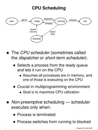
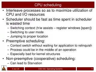
CPU Scheduler • The CPU Scheduler (short-term scheduler) selects a process in the ready queue and allocates a CPU to it. • CPU scheduling decisions may take place when a process: 1. Switches from running to waiting state 2. Switches from running to ready state 3. Switches from waiting to ready • Terminates • In situations 1 and 4, the process releases the CPU voluntarily. This is called nonpreemptive or cooperative scheduling. • In situations 2 and 3, the process is ready to run, but it does not have a CPU. This is called preemptive scheduling. • Problem: If a process is preempted while updating shared data, the system might be in an unstable state.
Dispatcher • The dispatchermodule gives control of the CPU to the process selected by the short-term scheduler. This involves: • Switching context • Switching to user mode • Jumping to the proper location in the user program to restart that program • Dispatch latency: time it takes for the dispatcher to stop one process and start another running
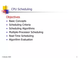
Scheduling Criteria How do we determine which CPU scheduling algorithm is best? Possible criteria: • CPU utilization: percent of time that the CPU is performing useful work • Throughput: number of processes that complete their execution per time unit • Turnaround time: amount of time to execute a particular process • Waiting time: amount of time a process has been waiting in the ready queue • Response time: amount of time it takes from when a request was submitted until the first response is produced
First-Come, First-Served (FCFS) Scheduling Suppose processes arrive in the order P1, P2, P3. P1 P2 P3 24 0 27 30 Average waiting time: (0 + 24 + 27)/3 = 17 milliseconds Suppose processes arrive in the order P2, P3, P1. P3 P2 P1 6 3 0 30 Average waiting time: (6 + 0 + 3)/3 = 3 milliseconds Convoy effect: many small processes wait for one big process to give up the CPU
Shortest-Job-First (SJF) Scheduling • Idea: associate with each process the length of its next CPU burst. Use these lengths to schedule the process with the shortest time. • SJF is optimal: it gives minimum average waiting time for a given set of processes. • The difficulty is knowing the length of the next CPU request. Example: P4 P1 P3 P2 16 9 0 3 24 • Average waiting time: (3 + 16 + 9 + 0) / 4 = 7
Length of Next CPU Burst • For a given process, can we estimate the length of the next CPU burst based on its previous CPU bursts? • An exponential average is commonly used: = actual length of CPU burst = predicted length of next CPU burst = parameter, , controls the influence of history • Note: • If , then history has no effect. • If , then only the most recent CPU burst matters
Length of Next CPU Burst Example: let and
Preemptive SJF Scheduling • If a new process arrives in the ready queue with a shorter expected CPU burst than the remaining expected time of the current process, the scheduler could preempt the current process. • This is called shortest-remaining-time-first scheduling. • Example: P1 P2 P1 P4 P3 17 5 0 1 10 26 • Average waiting time:
Priority Scheduling • A priority number (integer) is associated with each process. • The CPU is allocated to the process with the highest priority (assume that smallest integer corresponds to highest priority). • Priority scheduling can be either preemptive or nonpreemptive. • SJF is a priority scheduling where priority is the predicted next CPU burst time. • Example: P5 P2 P1 P3 P4 6 18 0 1 16 19 26 • Problem:Starvation– low priority processes may never execute • Solution: Aging– gradually increase priority of a process over time
Round Robin (RR) Scheduling • Each process gets a small unit of CPU time (time quantum), usually 10-100 milliseconds. After this time has elapsed, the process is preempted and added to the end of the ready queue. • If there are n processes in the ready queue and the time quantum is q, then each process gets 1/n of the CPU time in chunks of at most q time units at once. No process waits more than (n-1)q time units. • Example: Using a time quantum of 4 milliseconds: P1 P2 P3 P1 P1 P1 P1 P1 P1 34 22 30 14 18 4 10 0 7 26
Round Robin (RR) Scheduling • RR is basically FCFS with preemption • Performance • q large FCFS scheduling • q small each processes appears to have its own processor • Good performance requires that time quantum be large compared to the time required for switching context.
Practice Suppose the following processes arrive for execution at the times indicated, and they run for the times listed. With FCFS scheduling, what is the average waiting time and turnaround time? With nonpreemptive SJF scheduling, what is the average waiting time and turnaround time? Would the SJF results be different if process P2 arrived at time 0.0? What would happen if preemptive SJF scheduling is used?
Multilevel Queue • Ready queue is partitioned into separate queues, for example: • foreground (interactive) processes in one queue • background (batch) processes in another queue • Each queue has its own scheduling algorithm, for example: • foreground queue scheduled Round-Robin • background queue scheduled First-Come-First-Served • Scheduling must be done between the queues. Some possibilities: • Fixed priority scheduling: serve all foreground processes then background processes—possibility of starvation. • Time slice: each queue gets a certain amount of CPU time which it can schedule amongst its processes; e.g. 80% to foreground in RR and 20% to background in FCFS.
Multilevel Queue Scheduling Five-level priority example
Multilevel Feedback Queue • A process can move between the various queues depending on how it uses the CPU. • Aging can be implemented this way • A multilevel-feedback-queue scheduler is defined by the following parameters: • number of queues • scheduling algorithms for each queue • method used to determine when to upgrade a process • method used to determine when to demote a process • method used to determine which queue a process will enter when that process needs service
Examples of Multilevel Feedback Queue • Three queues: • Q0: highest priority; RR with time quantum 8 milliseconds • Q1: medium priority; RR time quantum 16 milliseconds • Q2: lowest priority; FCFS • Scheduling • A new job enters queue Q0which is servedRR. When it gains CPU, job receives 8 milliseconds. If it does not finish in 8 milliseconds, job is moved to queue Q1. • At Q1 job is again served RR and receives 16 additional milliseconds. If it still does not complete, it is preempted and moved to queue Q2.
Thread Scheduling • Operating system schedules kernel-level threads. • In the many-to-one and many-to-many models, the thread library schedules user-level threads to run on a LWP. • User-level thread scheduling is known as process-contention scope (PCS)since scheduling competition is within the process. • Kernel thread scheduled onto available CPU is system-contention scope (SCS) since competition is among all threads in system.
Multiple-Processor Scheduling • CPU scheduling is more complex when multiple CPUs are available. • Identical processors in a multiprocessor system are called homogeneous. • Asymmetric multiprocessing: only one processor handles scheduling, I/O processing, and system services • Symmetric multiprocessing (SMP): each processor is self-scheduling; all processes may be in common ready queue, or each may have its own private queue of ready processes • Most modern operating systems support SMP. • SMP implementations must ensure that shared data structures are handled responsibly.
Multiple-Processor Scheduling • If a process moves from one processor to another, the new processor’s cache must be updated with the process’ data. • Processor affinity: process has affinity for processor on which it is currently running • soft affinity: OS often, but not always, keeps a process running on the same processor • hard affinity: a process can specify that it must not migrate to a different processor • System architecture affects processor affinity, especially for non-uniform memory access (NUMA)
Multiple-Processor Scheduling • If each processor has its own private queue of processes, then some processors might be idle while others are busy. • Load balancing attempts to keep the workload evenly distributed across all processors in an SMP system. • Two general approaches: • Push migration: a specific task checks the load on each processor and redistributes (pushes) processes as necessary • Pull migration: an idle processor pulls a waiting task from a busy processor • Linux, for example, uses both pull and push migration. • Load balancing often counteracts the benefits of processor affinity.
Multicore Processors • Recent trend: multiple processor cores on same physical chip. • Faster and consumes less power than multiple chips. • Multiple threads per core: can take advantage of memory stall to make progress on another thread while memory retrieve happens Single thread running on a single processor: thread C M C M C M C M time C M compute cycle memory stall cycle Dual-threaded processor interleaving two processes: thread1 C M C M C M C M thread0 C M C M C M C M time
Example: Solaris Scheduling • Each thread belongs to one of six priority classes: real time, system, fair share, fixed priority, time sharing, and interactive • A real-time process runs before a process of any other class. • The system class runs kernel activities. • Each class includes its own set of priorities, which the scheduler converts to global priorities. • The scheduler selects the thread with the highest global priority, which runs until it blocks, uses its time slice, or is preempted by a higher-priority thread. • Higher priority threads are allocated smaller time slices.
Example: Solaris Scheduling Solaris dispatch table for time-sharing and interactive threads new priority of a thread that has used its entire time quantum without blocking (CPU-intensive) new priority of a thread that returns from sleep (e.g. waiting for I/O)
Example: Windows XP Scheduling • Windows XP uses priority-based preemptive scheduling. • 32 priority levels • Real-time class contains threads with priorities 16 to 31. • Variable classcontains threads with priorities 1-15. • A thread with priority 0 is used for memory management. • If no thread is ready to run, the system runs the idle thread. • If a process uses its entire time quantum, the system may lower its priority. • If a process waits for I/O, the system may raise its priority. • The window with which the user is currently interacting also gets a priority boost. • Windows tries to give good response time to processes that are using the mouse, keyboard, and windows.
Example: Windows XP Scheduling variable priority class relative priorities within a class default relative priority
Example: Linux Scheduling • Constant order O(1) scheduling time • Two priority ranges: • Real-timerange from 0 to 99 • Other tasks given a nicevalue from 100 to 140 • Lower values indicate higher priority • Higher-priority tasks get larger time slice than lower-priority tasks
Example: Linux Scheduling • Each processor maintains its own runqueueand schedules itself independently. • Each runqueue contains activeand expiredarrays, indexed by priority. • When all tasks have exhausted their time slices (i.e. active array is empty) the two arrays are interchanged.
Java Task Scheduling • JVM specification says that each thread has a priority, but does not specify how priorities and scheduling must be implemented. • If threads are time-sliced, then a runnable thread executes until: • Its time quantim expires • It blocks for I/O • It exits its run() method • Since some JVMs do not use time slices, a thread may give up the CPU via the yield() method • By calling the yield() method, the thread offers to let another process run; this is called cooperative multitasking. publicvoid run() { while (true) { // perform a CPU-intensive task ... // now yield control of the CPU Thread.yield(); } }
Java Task Scheduling • Each thread has an integer-value priority in a specified range • Threads inherit priority value of their parent • Thread priority can be set via the setPriority() method. • Priority of a Java thread is related to the priority of the kernel thread to which it is mapped. • Again, JVM implementations may implement prioritization however they chose.
Algorithm Evaluation • Deterministic modeling: takes a particular predetermined workload and determines the performance of each algorithm for that workload • Advantage: simple • Disadvantage: conclusions only apply for the specific workload considered • Queueingmodels: statistically describe the CPU and I/O bursts • Little’s formula: Let be the average queue length, the average waiting time, and the average arrival rate for new processes. If the system is stable, then: • Advantage: useful in comparing scheduling algorithms • Disadvantage: difficult to mathematically model complicated scheduling algorithms
Algorithm Evaluation • Simulations: program a model of the computer system; simulate processes, CPU bursts, I/O, etc.; observe the results • Trace tape: a record of the actual sequence of events in a real system, used as in put for a simulation • Advantage: can provide realistic results • Disadvantage: high cost of creating a simulator and running simulations • Implementation: implement the scheduling algorithm in the OS and see how it performs in practice • Advantage: it’s the only completely accurate way of evaluating a scheduling algorithm • Disadvantage: high cost; computing environments change over time