Sea-ice freeboard heights in the Arctic Ocean from ICESat and airborne laser

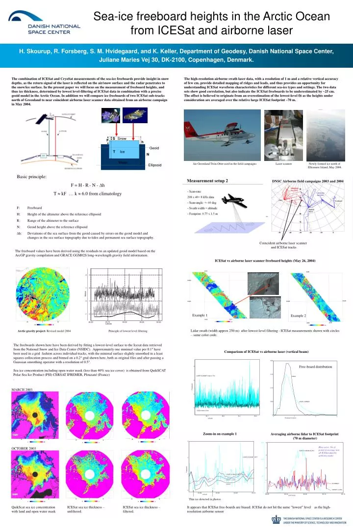
1. Snow S F h Geoid T Ice N Water Air Greenland Twin-Otter used in the field campaigns Laser scanner Newly formed ice north of Ellesmere Island, May 2004. Ellipsoid ICESat vs airborne laser scanner freeboard heights (May 26, 2004) Example 1 Example 2 Lidar swath (width approx 250 m) after lowest-level filtering - ICESat measurements shown with circles – same color code. Free-board distribution MARCH 2003 Thin ice detected in photos Blue curve: No of points in average (not all ICESat data hit airborne track) OCTOBER 2003 GREENICE May 2004 CRYOVEX April 2003 Alert Svalbard Station Nord QuikScat sea ice concentration with land and open water mask ICESat sea ice thickness – unfiltered. ICESat sea ice thickness – filtered. Sea-ice freeboard heights in the Arctic Oceanfrom ICESat and airborne laser H. Skourup, R. Forsberg, S. M. Hvidegaard, and K. Keller, Department of Geodesy, Danish National Space Center, Juliane Maries Vej 30, DK-2100, Copenhagen, Denmark. The combination of ICESat and CryoSat measurements of the sea-ice freeboards provide insight in snow depths, as the return signal of the laser is reflected on the air/snow surface and the radar penetrates to the snow/ice surface. In the present paper we will focus on the measurement of freeboard heights, and thus ice thickness, determined by lowest level-filtering of ICESat data in combination with a precise geoid model in the Arctic Ocean. In addition we will compare ice freeboards of two ICESat sub-tracks north of Greenland to near coincident airborne laser scanner data obtained from an airborne campaign in May 2004. The high-resolution airborne swath laser data, with a resolution of 1 m and a relative vertical accuracy of few cm, provide detailed mapping of ridges and leads, and thus provides an opportunity for understanding ICESat waveform characteristics for different sea-ice types and settings. The two data sets show good correlation, but also indicate the ICESat freeboards to be underestimated by ~25 cm. The offset is believed to originate from an overestimation of the lowest-level fit as the heights under consideration are averaged over the relative large ICESat footprint ~70 m. Basic principle: F=H- R- N-h T  kF … k  6.0 from climatology F: Freeboard H: Height of the altimeterabove the reference ellipsoid R: Range of thealtimeter to the surface N: Geoid height above thereference ellipsoid h: Deviations of the sea surfacefrom the geoid caused by errors on the geoid model and changes inthe sea surface topography due to tides and permanent sea surfacetopography. DNSC Airborne field campaigns 2003 and 2004 Coincident airborne laser scanner and ICESat tracks The freeboard values have been derived using the residuals to an updated geoid model based on the ArcGP gravity compilation and GRACE GGM02S long-wavelength gravity field information.   Nadir-looking imagery Arctic gravity project: Revised model 2004 Principle of lowest level filtering The freeboards shown here have been derived by fitting a lowest-level surface to the Icesat data retrieved from the National Snow and Ice Data Center (NSIDC). Approximately one minimal value per 0.1 have been used in a grid fashion across individual tracks, with the minimal surface slightly smoothed in a least squares collocation process and binned on a 0.2 grid shown here, both as original files and after passing a Gaussian smoothing operator with a resolution of 0.5. Sea ice concentration including open water mask (less than 40% sea ice cover) is obtained from QuikSCAT Polar Sea Ice Product (PSI) CERSAT IFREMER, Plouzané (France) . Comparison of ICESat vs airborne laser (vertical beam) Zoom-in on example 1 Averaging airborne lidar to ICESat footprint (70 m diameter) It appears that ICESat free-boards are biased. ICESat do not hit the same ”lowest” level as the high-resolution airborne sensor