Download
1 / 33
330 likes | 478 Views
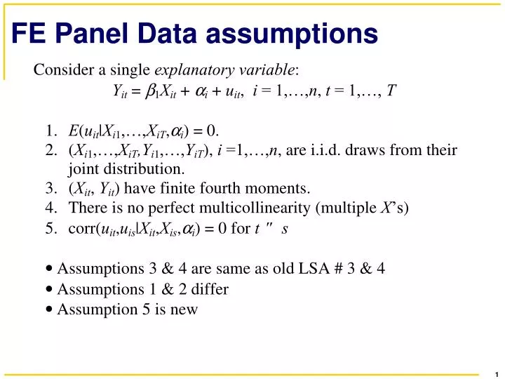
FE Panel Data assumptions. Assumption #1: E ( u it | X i 1 ,…, X iT , i ) = 0 . Assumption #2: ( X i 1 ,…, X iT ,Y i 1 ,…, Y iT ), i =1,…, n , are i.i.d. draws from their joint distribution . Assumption #5: corr( u it , u is | X it , X is , i ) = 0 for t ≠ s.

E N D
Assumption #2: (Xi1,…,XiT,Yi1,…,YiT), i =1,…,n, are i.i.d. draws from their joint distribution
. use fatality . xtset state year panel variable: state (strongly balanced) time variable: year, 1982 to 1988 delta: 1 unit . gen vfr = mrall*10000 . xtreg vfr beertax, fe Fixed-effects (within) regression Number of obs = 336 Group variable: state Number of groups = 48 R-sq: within = 0.0407 Obs per group: min = 7 between = 0.1101 avg = 7.0 overall = 0.0934 max = 7 F(1,287) = 12.19 corr(u_i, Xb) = -0.6885 Prob > F = 0.0006 ------------------------------------------------------------------------------ vfr | Coef. Std. Err. t P>|t| [95% Conf. Interval] -------------+---------------------------------------------------------------- beertax | -.6558736 .18785 -3.49 0.001 -1.025612 -.2861352 _cons | 2.377075 .0969699 24.51 0.000 2.186212 2.567937 -------------+---------------------------------------------------------------- sigma_u | .7147146 sigma_e | .18985942 rho | .93408484 (fraction of variance due to u_i) ------------------------------------------------------------------------------ F test that all u_i=0: F(47, 287) = 52.18 Prob > F = 0.0000 . estimates store figs
. xtreg vfr beertax, re Random-effects GLS regression Number of obs = 336 Group variable: state Number of groups = 48 R-sq: within = 0.0407 Obs per group: min = 7 between = 0.1101 avg = 7.0 overall = 0.0934 max = 7 Random effects u_i ~ Gaussian Wald chi2(1) = 0.18 corr(u_i, X) = 0 (assumed) Prob > chi2 = 0.6753 ------------------------------------------------------------------------------ vfr | Coef. Std. Err. z P>|z| [95% Conf. Interval] -------------+---------------------------------------------------------------- beertax | -.0520158 .1241758 -0.42 0.675 -.2953959 .1913643 _cons | 2.067141 .0999715 20.68 0.000 1.871201 2.263082 -------------+---------------------------------------------------------------- sigma_u | .5157915 sigma_e | .18985942 rho | .88067496 (fraction of variance due to u_i) ------------------------------------------------------------------------------ . estimates store rutabagas . hausman figs rutabagas ---- Coefficients ---- | (b) (B) (b-B) sqrt(diag(V_b-V_B)) | figs rutabagas Difference S.E. -------------+---------------------------------------------------------------- beertax | -.6558736 -.0520158 -.6038579 .1409539 ------------------------------------------------------------------------------ b = consistent under Ho and Ha; obtained from xtreg B = inconsistent under Ha, efficient under Ho; obtained from xtreg Test: Ho: difference in coefficients not systematic chi2(1) = (b-B)'[(V_b-V_B)^(-1)](b-B) = 18.35 Prob>chi2 = 0.0000
What if Assumption #5 fails: so corr(uit,uis|Xit,Xis,i) ≠ 0?
Remember, we should use xtreg: . xtreg vfr beertax yr2 yr3 yr4 yr5 yr6 yr7, fe vce(cluster state) Fixed-effects (within) regression Number of obs = 336 Group variable: state Number of groups = 48 R-sq: within = 0.0803 Obs per group: min = 7 between = 0.1101 avg = 7.0 overall = 0.0876 max = 7 F(7,47) = 4.36 corr(u_i, Xb) = -0.6781 Prob > F = 0.0009 (Std. Err. adjusted for 48 clusters in state) ------------------------------------------------------------------------------ | Robust vfr | Coef. Std. Err. t P>|t| [95% Conf. Interval] -------------+---------------------------------------------------------------- beertax | -.6399799 .3570783 -1.79 0.080 -1.358329 .0783691 yr2 | -.0799029 .0350861 -2.28 0.027 -.1504869 -.0093188 yr3 | -.0724206 .0438809 -1.65 0.106 -.1606975 .0158564 yr4 | -.1239763 .0460559 -2.69 0.010 -.2166288 -.0313238 yr5 | -.0378645 .0570604 -0.66 0.510 -.1526552 .0769262 yr6 | -.0509021 .0636084 -0.80 0.428 -.1788656 .0770615 yr7 | -.0518038 .0644023 -0.80 0.425 -.1813645 .0777568 _cons | 2.42847 .2016885 12.04 0.000 2.022725 2.834215 -------------+---------------------------------------------------------------- sigma_u | .70945965 sigma_e | .18788295 rho | .93446372 (fraction of variance due to u_i) ------------------------------------------------------------------------------ • Exact same as , fe robust !!! Stata version 9 incorrect! Stata 10, 11 good • Stock & Watson (2008), “Heteroskedasticity-Robust Standard Errors for Fixed Effect Panel Data Regression,”Econometrica, 76 (1): 155 – 74.
Application: Drunk Driving Laws and Traffic Deaths (Ruhm, J. Health Econ, 1996)