Download
1 / 128
1.29k likes | 1.43k Views
Elena Maftei Technical University of Denmark DTU Informatics. Synthesis of Digital Microfluidic Biochips with Reconfigurable Operation Execution. www.dreamstime.com. Digital Microfluidic Biochip. Duke University. Applications. Sampling and real time testing of

E N D
Elena MafteiTechnical University of Denmark DTU Informatics Synthesis of Digital Microfluidic Biochips with Reconfigurable Operation Execution www.dreamstime.com
Digital Microfluidic Biochip Duke University
Applications • Sampling and real time testing of air/water for biochemical toxins • Food testing • DNA analysis and sequencing • Clinical diagnosis • Point of care devices • Drug development
Advantages & Challenges • Advantages: • High throughput (reduced sample / reagent consumption) • Space (miniaturization) • Time (parallelism) • Automation (minimal human intervention) • Challenges: • Design complexity • Radically different design and test methods required • Integration with microelectronic components in future SoCs
Outline • Motivation • Architecture • Operation Execution • Contribution I • Module-Based Synthesis with Dynamic Virtual Devices • Contribution II • Routing-Based Synthesis • Contribution III • Droplet-Aware Module-Based Synthesis • Conclusions & Future Directions
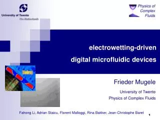
R2 Ground electrode Top plate B Droplet Insulators Filler fluid S2 Bottom plate S3 Control electrodes R1 S1 W Architecture and Working Principles Biochip architectureCell architecture Reservoir • Electrowetting-on-dielectric Detector
Microfluidic Operations R2 B S2 S3 R1 S1 W • Dispensing • Detection • Splitting/Merging • Storage • Mixing/Dilution
R2 B S2 S3 R1 S1 W Reconfigurability • Dispensing • Detection • Splitting/Merging • Storage • Mixing/Dilution
R2 B S2 S3 R1 S1 W Reconfigurability Non-reconfigurable • Dispensing • Detection • Splitting/Merging • Storage • Mixing/Dilution
R2 B S2 S3 R1 S1 W Reconfigurability Non-reconfigurable • Dispensing • Detection • Splitting/Merging • Storage • Mixing/Dilution Reconfigurable
R2 B S2 S3 R1 S1 W Module-Based Operation Execution 2 x 4 module
R2 B S2 S3 R1 S1 W Module-Based Operation Execution 2 x 4 module Module library
R2 B S2 S3 R1 S1 W Module-Based Operation Execution 2 x 4 module segregation cells
R2 B S2 S3 R1 S1 W Module-Based Operation Execution • Operations confined to rectangular, fixed modules • Positions of droplets inside modules ignored • Segregation cells
S3 B1 1 2 3 4 In B In S1 In S2 In R1 5 6 S1 R2 Dilute Mix 7 8 9 10 11 In S3 In R2 In B In B S2 R1 D1 12 13 Dilute Dilute B2 W Example Application graph t
S3 B1 1 2 3 4 S2 R1 S1 B1 5 6 S1 R2 2 x 2 2 x 4 7 2 x 4 8 9 10 11 S2 R1 S3 B1 R2 B2 D1 12 13 2 x 2 2 x 2 B2 W Example Application graph Biochip
S3 B1 1 2 3 4 S2 R1 S1 B1 5 6 S1 R2 2 x 2 2 x 4 7 2 x 4 8 9 10 11 S2 R1 S3 B1 R2 B2 D1 12 13 2 x 2 2 x 2 B2 W Example D2(O5) Application graph t
S3 B1 1 2 3 4 S2 R1 S1 B1 5 6 S1 R2 2 x 2 2 x 4 7 2 x 4 8 9 10 11 S2 R1 S3 B1 R2 B2 12 13 2 x 2 2 x 2 B2 W Example D4 (O13) store O5 D3 (O12) M1 (O6) Application graph t+4
S3 B1 1 2 3 4 S2 R1 S1 B1 5 6 S1 R2 2 x 4 2 x 2 7 2 x 4 8 9 10 11 S2 R1 S3 B1 R2 B2 12 13 2 x 2 2 x 2 B2 W Example D4 (O13) M2(O7) D3 (O12) Application graph t+8
1 2 3 4 S2 R1 S1 B1 t t+8 t+11 Allocation 5 6 2 x 2 2 x 4 O6 Mixer1 store Diluter2 O5 7 2 x 4 8 9 10 11 O7 Mixer2 S3 B1 R2 B2 Diluter3 O12 12 13 O13 Diluter4 2 x 2 2 x 2 Example Application graph Schedule
S3 B1 1 2 3 4 S2 R1 S1 B1 D2(O5) 5 6 S1 R2 2 x 4 2 x 2 7 2 x 4 8 9 10 11 S2 R1 S3 B1 R2 B2 D1 12 13 2 x 2 2 x 2 B2 W Example Application graph t
S3 B1 1 2 3 4 S2 R1 S1 B1 D2(O5) 5 6 S1 R2 2 x 4 2 x 2 7 2 x 4 8 9 10 11 S2 R1 S3 B1 R2 B2 12 13 2 x 2 2 x 2 B2 W Example Application graph t
S3 B1 1 2 3 4 S2 R1 S1 B1 D2(O5) 5 6 S1 R2 2 x 4 2 x 2 7 2 x 4 8 9 10 11 S2 R1 S3 B1 R2 B2 12 13 2 x 2 2 x 2 B2 W Example Application graph t
S3 B1 1 2 3 4 S2 R1 S1 B1 D2(O5) 5 6 S1 R2 2 x 4 2 x 2 7 2 x 4 8 9 10 11 S2 R1 S3 B1 R2 B2 12 13 2 x 2 2 x 2 B2 W Example Application graph t
S3 B1 1 2 3 4 S2 R1 S1 B1 D2(O5) 5 6 S1 R2 2 x 4 2 x 2 7 2 x 4 8 9 10 11 S2 R1 S3 B1 R2 B2 12 13 2 x 2 2 x 2 B2 W t Example Application graph
S3 B1 1 2 3 4 S2 R1 S1 B1 D2(O5) 5 6 S1 R2 2 x 4 2 x 2 7 2 x 4 8 9 10 11 S2 R1 S3 B1 R2 B2 12 13 2 x 2 2 x 2 B2 W t Example Application graph
S3 B1 1 2 3 4 S2 R1 S1 B1 D2(O5) 5 6 S1 R2 2 x 4 2 x 2 7 2 x 4 8 9 10 11 S2 R1 S3 B1 R2 B2 12 13 2 x 2 2 x 2 B2 W t Example Application graph
S3 B1 1 2 3 4 S2 R1 S1 B1 D2(O5) 5 6 S1 R2 2 x 4 2 x 2 7 2 x 4 8 9 10 11 S2 R1 S3 B1 R2 B2 12 13 2 x 2 2 x 2 B2 W t Example Application graph
S3 B1 1 2 3 4 S2 R1 S1 B1 D2(O5) 5 6 S1 R2 2 x 4 2 x 2 7 2 x 4 8 9 10 11 S2 R1 S3 B1 R2 B2 12 13 2 x 2 2 x 2 B2 W t Example Application graph
S3 B1 1 2 3 4 S2 R1 S1 B1 D2(O5) 5 6 S1 R2 2 x 4 2 x 2 7 2 x 4 8 9 10 11 S2 R1 S3 B1 R2 B2 12 13 2 x 2 2 x 2 B2 W t Example Application graph
S3 B1 1 2 3 4 S2 R1 S1 B1 D2(O5) 5 6 S1 R2 2 x 4 2 x 2 7 2 x 4 8 9 10 11 S2 R1 S3 B1 R2 B2 12 13 2 x 2 2 x 2 B2 W t Example Application graph
S3 B1 1 2 3 4 S2 R1 S1 B1 D2(O5) 5 6 S1 R2 2 x 4 2 x 2 7 2 x 4 8 9 10 11 S2 R1 S3 B1 R2 B2 D1 12 13 2 x 2 2 x 2 B2 W t Example Application graph
S3 B1 1 2 3 4 S2 R1 S1 B1 D2(O5) 5 6 S1 R2 2 x 4 2 x 2 7 2 x 4 8 9 10 11 S2 R1 S3 B1 R2 B2 D1 12 13 2 x 2 2 x 2 B2 W t Example M1 (O6) Application graph
S3 B1 1 2 3 4 S2 R1 S1 B1 D4 (O13) 5 6 S1 R2 2 x 4 2 x 2 7 2 x 4 8 9 10 11 M2 (O7) S2 R1 D3 (O12) S3 B1 R2 B2 12 13 2 x 2 2 x 2 B2 W Example Application graph t+4
t t+8 t+11 Allocation O6 Mixer1 store Diluter2 O5 O7 Mixer2 Diluter3 O12 O13 Diluter4 Example t t+4 t+9 Allocation O6 Mixer1 Diluter2 O5 Mixer2 O7 Diluter3 O12 O13 Diluter4 Schedule – operation execution with fixed virtual modules Schedule – operation execution with dynamic virtual modules
Solution Tabu Search • Binding of modules to operations • Schedule of the operations • Placement of modules performed inside scheduling • Placement of the modules • Free space manager based on [Bazargan et al. 2000] that divides free space on the chip into overlapping rectangles List Scheduling Maximal Empty Rectangles
S3 B1 S1 R1 S2 R2 B2 W Dynamic Placement Algorithm (3,8) (8,8) Rect2 Rect3 Rect1 (0,4) D1 (0,0) (7,0)
S3 B1 S1 R1 S2 R2 B2 W Dynamic Placement Algorithm (8,8) Rect2 D2(O5) (6,4) Rect3 (3,4) Rect1 D1 (0,0) (7,0)
S3 B1 S1 R1 S2 R2 B2 W Dynamic Placement Algorithm (8,8) D2(O5) Rect2 (8,4) Rect1 D1 (4,0) (6,0)
Experimental Evaluation • Tabu Search-based algorithm implemented in Java • Benchmarks • Real-life applications • Colorimetric protein assay • In-vitro diagnosis • Polymerase chain reaction – mixing stage • Synthetic benchmarks • 10 TGFF-generated benchmarks with 10 to 100 operations • Comparison between: • Module-based synthesis with fixed modules (MBS) • T-Tree [Yuh et al. 2007] • Module-based synthesis with dynamic modules (DMBS)
Area Time limit (min) Best (s) Average (s) Standard dev. (%) 13 x 13 60 182 189.99 2.90 10 182 192.00 3.64 1 191 199.20 4.70 12 x 12 60 182 190.86 3.20 10 185 197.73 6.50 1 193 212.62 10.97 60 184 192.50 3.78 10 194 211.72 14.37 1 226 252.19 15.76 Experimental Evaluation Best-, average schedule length and standard deviation out of 50 runs for MBS Colorimetric protein assay Colorimetric protein assay Colorimetric protein assay Colorimetric protein assay
Experimental Evaluation Best schedule length out of 50 runs for MBS vs. T-Tree Colorimetric protein assay Colorimetric protein assay Colorimetric protein assay Colorimetric protein assay Colorimetric protein assay Colorimetric protein assay Colorimetric protein assay 22.91 % improvement for 9 x 9
Experimental Evaluation Average schedule length out of 50 runs for DMBS vs. MBS Colorimetric protein assay Colorimetric protein assay Colorimetric protein assay Colorimetric protein assay Colorimetric protein assay 7.68 % improvement for 11 x 12
R2 R2 B B c1 S2 S2 c2 S3 S3 R1 R1 S1 W S1 W Module-Based vs. Routing-Based Operation Execution
R2 B 180◦ c1 S2 c2 S3 90◦ 90◦ 0◦ R1 S1 W Operation Execution Characterization p90, p180, p0 ?
180◦ 0◦ 0◦ 90◦ 0◦ 0◦ 90◦ 90◦ 90◦ 0◦ 0◦ 0◦ 0◦ 180◦ 90◦ 0◦ 90◦ 90◦ 90◦ 90◦ 90◦ 90◦ 0◦ 90◦ Operation Execution Characterization p90, p180, p0 Electrode pitch size = 1.5 mm, gap spacing = 0.3 mm, average velocity rate = 20 cm/s.
Operation Execution Characterization p90 = 0.1 % p180 = - 0.5 % p0 = 0.29 % p0 = 0.58 % 1 2 Electrode pitch size = 1.5 mm, gap spacing = 0.3 mm, average velocity rate = 20 cm/s.
R2 B 4 1 2 3 5 6 In R2 In S3 In B In R1 In S1 In S2 S2 8 9 7 Dilute S3 Mix Mix 11 In R1 R1 10 12 13 Waste Mix Mix S1 W Example Application graph Biochip