TSpectrum class developments
620 likes | 634 Views
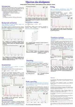
Miroslav Morháč Institute of Physics, Slovak Academy of Sciences, Bratislava, Slovakia. TSpectrum class developments. ROOT 2005 Workshop, September 28-30, CERN Geneva. Introduction. TSpectrum class of the ROOT system is an efficient tool aimed for the analysis of spectra

TSpectrum class developments
E N D
Presentation Transcript
Miroslav Morháč Institute of Physics, Slovak Academy of Sciences, Bratislava, Slovakia TSpectrum class developments ROOT 2005 Workshop, September 28-30, CERN Geneva
Introduction • TSpectrum class of the ROOT system is an efficient tool aimed for the analysis of spectra • (histograms) from the experiments in nuclear, high energy physics (possibly other types of data) • it includes non-conventional processing functions of • background estimation, elimination • deconvolution – resolution improvement • smoothing • peak identification • fitting • orthogonal transforms, filtering, enhancement Aim of the talk • to present the set of functions implemented in TSpectrum class • to explain briefly, the principles of the mathematical methods implemented in TSpectrum class • to explain the meaning of individual parameters in the calls of TSpectrum functions • to give few examples of how to use the functions in TSpectrum and illustrating the influence of • the parameters • to outline possible improvements, modifications, and extensions to TSpectrum2, 3
Background estimation Goal: Separation of useful information (peaks) from useless information (background) • method is based on Sensitive Nonlinear Iterative Peak (SNIP) clipping algorithm • new value in the channel “i” is calculated where p = 1, 2, …, number_of_iterations. In fact it represents second order difference filter (-1,2,-1) Function 1: const char* Background1(float *spectrum, int size, int number_of_iterations) Parameters • spectrum-pointer to the vector of source spectrum • size-length of the source spectrum • number_of_iterations or width of the clipping window This function calculates background spectrum from the source spectrum. The result is placed in the vector pointed by spectrum pointer. On successful completion it returns 0. On error it returns pointer to the string describing error.
Example 1– script Background1.c : Figure 1 Example of the estimation of background for number_of_iterations=6. Original spectrum is shown in black color, estimated background in red color.
Function 2: const char* Background1General(float *spectrum, int size, int number_of_iterations, int direction, int filter_order, bool compton) Parameters • spectrum-pointer to the vector of source spectrum • size-length of the source spectrum • number_of_iterations or width of the clipping window • direction- direction of change of clipping window - possible values: BACK1_INCREASING_WINDOW • BACK1_DECREASING_WINDOW • filter_order-order of clipping filter - possible values: • BACK1_ORDER2 • BACK1_ORDER4 • BACK1_ORDER6 • BACK1_ORDER8 • compton- logical variable whether the estimation of Compton edge will be included BACK1_EXCLUDE_COMPTON BACK1_INCLUDE_COMPTON It represents generalization of the previous function. The meaning of the first three parameters is the same. Moreover one can change the direction of the change of the clipping window, the order of the clipping filter and to include the estimation of Compton edges.
One can notice that in Figure 1 at the edges of the peaks the estimated background goes under the peaks. An alternative approach is to decrease the clipping window from a given value number_of_iterations to the value of one (DECREASING CLIPPING WINDOW) is presented in Example 2. Example 2 – script Background1General_decr.c : Figure 2 Example of the estimation of background for number_of_iterations=6 using decreasing clipping window algorithm. Original spectrum is shown in black color, estimated background in red color.
the question is how to choose the width of the clipping window, i.e., number_of_iterations parameter. The influence of this parameter on the estimated background is illustrated in Figure 3. Example 3 – script Background1General_width.c : Figure 3 Example of the influence of clipping window width on the estimated background for number_of_iterations=4 (red line), 6 (blue line) 8 (green line) using decreasing clipping window algorithm. • in general one should set this parameter so that the value 2*number_of_iterations+1 was greater than the widths of preserved objects (peaks).
another example for very complex spectrum Figure 4. Example 4 – script Background1General_width2.c : Figure 4 Example of the influence of clipping window width on the estimated background for number_of_iterations=10 (red line), 20 (blue line), 30 (green line) and 40 (magenta line) using decreasing clipping window algorithm.
second order difference filter removes linear (quasi-linear) background and preserves symmetrical peaks. • however if the shape of the background is more complex one can employ higher-order clipping filters (see example in Figure 5) Example 5 – script Background1General_order.c : Figure 5 Example of the influence of clipping filter difference order on the estimated background for number_of_iterations=40, 2-nd order red line, 4-th order blue line, 6-th order green line and 8-th order magenta line, and using decreasing clipping window algorithm.
sometimes it is necessary to include also the Compton edges into the estimate of the background. In Figure 6 we present the example of the synthetic spectrum with Compton edges. • the background was estimated using the 8-th order filter with the estimation of the Compton edges and decreasing clipping window. Example 6 – script Background1General_compton.c : Figure 6 Example of the estimate of the background with Compton edges (red line) for number_of_iterations=40, 8-th order difference filter and using decreasing clipping window algorithm.
References: [1] C. G Ryan et al.: SNIP, a statistics-sensitive background treatment for the quantitative analysis of PIXE spectra in geoscience applications. NIM, B34 (1988), 396-402. [2] M. Morháč, J. Kliman, V. Matoušek, M. Veselský, I. Turzo.: Background elimination methods for multidimensional gamma-ray spectra. NIM, A401 (1997) 113-132. [3] D. D. Burgess, R. J. Tervo: Background estimation for gamma-ray spectroscopy. NIM 214 (1983), 431-434. Possible extension of TSpectrum background estimation method: • the estimate of the background can be influenced by noise present in the spectrum. We proposed • the algorithm of the background estimate with simultaneous smoothing • in the original algorithm without smoothing, the estimated background snatches the lower spikes in • the noise. Consequently, the areas of peaks are biased by this error. Figure 7 Illustration of non-smoothing and smoothing algorithm of background estimation
Deconvolution Goal: Improvement of the resolution in spectra, decomposition of multiplets Mathematical formulation of the convolution system is where h(i) is the impulse response function, x, y are input and output vectors, respectively, N is the length of x and h vectors. In matrix form we have
let us assume that we know the response and the output vector (spectrum) of the above given • system. • the deconvolution represents solution of the overdetermined system of linear equations, i.e., • the calculation of the vector x. • from numerical stability point of view the operation of deconvolution is extremely critical (ill-posed • problem) as well as time consuming operation. • the Gold deconvolution algorithm proves to work very well, other methods (Fourier, VanCittert etc) • oscillate. • it is suitable to process positive definite data (e.g. histograms). Gold deconvolution algorithm where l is given number of iterations
Function 3: const char* Deconvolution1(float *source, const float *resp, int size, int number_of_iterations) This function calculates deconvolution from source spectrum according to response spectrum The result is placed in the vector pointed by source pointer. Parameters • source - pointer to the vector of source spectrum • resp - pointer to the vector of response spectrum • size - length of the source and response spectra • number_of_iterations – parameter l in the Gold deconvolution algorithm Figure 8 Source spectrum Figure 9 Response spectrum
response function (usually peak) should be shifted left to the first non-zero channel (bin) (see • Figure 9) Figure 10 Principle how the response matrix is composed inside of the Deconvolution1 function
Example 7 – script Deconvolution1.c : Figure 11 Example of Gold deconvolution. The original source spectrum is drawn with black color, the spectrum after the deconvolution (10000 iterations) with red color,
further let us study the influence of the number of iterations on the deconvolved spectrum (Figure 12) Example 8 – script Deconvolution1_iter.c : Figure 12 Study of Gold deconvolution algorithm. The original source spectrum is drawn with black color, spectrum after 100 iterations with red color,spectrum after 1000 iterations with blue color,spectrum after 10000 iterations with green color and spectrum after 100000 iterations with magenta color.
Set the initial solution Boosted deconvolution 2. Set required number of repetitions and iterations 3. Set the number of repetitions find solution 4. Using Gold deconvolution algorithm for • stop calculation, else • apply boosting operation, i.e., set 5. If ; is boosting coefficient >0 and b. c. continue in 4. Function 4: const char* Deconvolution1HighResolution(float *source, const float *resp, int size, int number_of_iterations, int number_of_repetitions, double boost) This function calculates deconvolution from source spectrum according to response spectrum using boosted Gold deconvolution algorithm. The result is placed in the vector pointed by source pointer.
Parameters • source - pointer to the vector of source spectrum • resp - pointer to the vector of response spectrum • size - length of the source and response spectra • number_of_iterations - parameter L in the boosted Gold deconvolution algorithm • number_of_repetitions - parameter R in the boosted Gold deconvolution algorithm • boost – boosting coefficient p (should be >0, recommended range <1, 2>) Example 9 – script Deconvolution1_hr.c : Figure 13 Example of boosted Gold deconvolution. The original source spectrum is drawn with black color, deconvolved spectrum (200 iterations, 50 repetitions, p=1.2) with red color.
for relatively narrow peaks in the above given example the Gold deconvolution method combined with boosting operation (Deconvolution1HighResolution function) is able to decompose overlapping peaks practically to delta - functions. • in the next example we have chosen a synthetic data (spectrum, 256 channels) consisting of 5 very closely positioned, relatively wide peaks (sigma =5), with added noise (Figure 14). • thin lines represent pure Gaussians (see Table 1); thick line is a resulting spectrum with additive noise (10% of the amplitude of small peaks). Table 1 Positions, heights and areas of peaks in the spectrum shown in Figure 14 Figure 14 Testing example of synthetic spectrum composed of 5 Gaussians with added noise
in ideal case, we should obtain the result given in Figure 15. The areas of the Gaussian components of the spectrum are concentrated completely to delta -functions • when solving the overdetermined system of linear equations with data from Figure 14 in the sense of minimum least squares criterion without any regularization we obtain the result with large oscillations (Figure 16). • from mathematical point of view, it is the optimal solution in the unconstrained space of independent variables. From physical point of view we are interested only in a meaningful solution. • therefore, we have to employ regularization techniques (e.g. Gold deconvolution) and/or to confine the space of allowed solutions to subspace of positive solutions. Figure 16 Least squares solution of the system of linear equations without regularization Figure 15 The same spectrum like in Figure 14, outlined bars show the contents of present components (peaks)
Example 10 – script Deconvolution1_wide.c : Figure 17 The original source spectrum is drawn with black color, deconvolved spectrum using classic Gold deconvolution (10000 iterations) with red color, deconvolved spectrum using classic high resolution Gold deconvolution (200 iterations, 50 repetitions, p=1.2) with blue color.
Decomposition - unfolding Function 5: const char* Deconvolution1Unfolding(float *source, const float **resp, int sizex, int sizey, int number_of_iterations) This function unfolds source spectrum according to response matrix columns. The result is placed in the vector pointed by source pointer. Parameters • source - pointer to the vector of source spectrum • resp - pointer to the matrix of response spectra • sizex - length of source spectrum and # of columns in response matrix • sizey - length of destination spectrum and # of rows in response matrix • number_of_iterations – parameter l in the Gold deconvolution algorithm • Note!!! sizex must be >= sizey After decomposition the resulting channels are written back to the first sizey channels of the source spectrum.
Figure 18 Response matrix composed of neutron spectra of pure chemical elements
Example 11 – script Deconvolution1Unfolding.c : Figure 20 Spectrum after decomposition, contains 10 coefficients, which correspond to contents of chemical components (dominant 8-th and 10-th components, i.e. O, Si) Figure 19 Source neutron spectrum to be decomposed References: [1] Gold R., ANL-6984, Argonne National Laboratories, Argonne Ill, 1964. [2] Coote G.E., Iterative smoothing and deconvolution of one- and two-dimensional elemental distribution data, NIM B 130 (1997) 118. [3] M. Morháč, J. Kliman, V. Matoušek, M. Veselský, I. Turzo.: Efficient one- and two-dimensional Gold deconvolution and its application to gamma-ray spectra decomposition. NIM, A401 (1997) 385-408. [4] Morháč M., Matoušek V., Kliman J., Efficient algorithm of multidimensional deconvolution and its application to nuclear data processing, Digital Signal Processing 13 (2003) 144.
Possible new TSpectrum deconvolution methods: • one-fold Gold deconvolution and its boosted version (see e.g. M. Morháč,Deconvolution methods and their applications in the analysis of gamma-ray spectra, ACAT2005, May 22-27, Zeuthen Germany) Figure 21 Original spectrum (thick line) and deconvolved spectrum using one-fold Gold algorithm ( 10000 iterations, thin line) Figure 22 Illustration of deconvolution via boosted Gold deconvolution Table 2 Results of the estimation of peaks in spectrum shown in Figure 22
Richardson – Lucy deconvolution and its boosted version -see e.g. • Lucy L.B., A.J. 79 (1974) 745. • Richardson W.H., J. Opt. Soc. Am. 62 (1972) 55. Figure 23 Illustration of application of Richardson-Lucy algorithm of deconvolution Figure 24 Spectrum deconvolved using boosted Richardson-Lucy algorithm of deconvolution Table 3 Results of the estimation of peaks in spectrum shown in Figure 24
Smoothing Goal: Suppression of statistical fluctuations • there exist enormous number of filtration techniques • we mention Markov smoothing algorithm, which can be employed for the identification of peaks in noisy spectra • the algorithm is based on discrete Markov chain, which has very simple invariant distribution being defined from the normalization condition n is the length of the smoothed spectrum and is the probability of the change of the peak position from channel I to the channel i+1. is the normalization constant so that and m is a width of smoothing window.
Function 6: const char* TSpectrum::Smooth1Markov(float *source, int size, int aver_window) This function calculates smoothed spectrum from the source spectrum based on Markov chain method. The result is placed in the vector pointed by source pointer. • Parameters • source - pointer to the vector of source spectrum • size - length of source spectrum • aver_window - width of averaging smoothing window Reference: [1] Z.K. Silagadze, A new algorithm for automatic photopeak searches. NIM A 376 (1996), 451.
Example 12 – script Smoothing1.c : Example 13 – script Smoothing2.c : Figure 25 Original noisy spectrum Figure 26 Smoothed spectrum m=3 Example 14 – script Smoothing3.c : Example 15 – script Smoothing4.c : Figure 27 Smoothed spectrum m=7 Figure 28 Smoothed spectrum m=10
Peaks searching Goal: to identify automatically the peaks in a spectrum with the presence of the continuous background and statistical fluctuations - noise. • The common problems connected with correct peak identification are • non-sensitivity to noise, i.e., only statistically relevant peaks should be identified. • non-sensitivity of the algorithm to continuous background. • ability to identify peaks close to the edges of the spectrum region. Usually peak finders fail to detect them. • resolution, decomposition of doublets and multiplets. The algorithm should be able to recognize close positioned peaks. • ability to identify peaks with different sigma General peak searching algorithm based on smoothed second differences – implemented in Search1 function in old versions of ROOT (up to the Version 3.04) • it is based on smoothed second differences (SSD) that are compared to its standard deviations . Figure 29 Smoothed Second Differences (SSD) and its standard deviation in the vicinity of peak
Figure30 Synthetic spectrum and its SSD spectrum Figure31 An example of one-dimensional gamma-ray experimental spectrum with found peaks and its inverted positive SSD spectrum
High resolution peak searching algorithm • it is based on the above presented Gold deconvolution algorithm • unlike SSD algorithm before applying the deconvolution algorithm we have to remove the background using one of the above presented background elimination algorithms • if desired, before applying the peak searching algorithm the Markov smoothed spectrum (described in previous section) can be calculated as well Function 7: Int_tSearch(TH1 * hin, Double_t sigma, Option_t * option, Double_t threshold) This function searches for peaks in source spectrum in hin The number of found peaks and their positions are written into the members fNpeaks and fPositionX. The search is performed in the current histogram range. • Parameters • hin - pointer to the histogram of source spectrum • sigma - sigma of searched peaks • option - if option is not equal to "goff" (goff is the default), then a polymarker object is created and added to the list of functions of the histogram. The histogram is drawn with the specified option and the polymarker object drawn on top of the histogram. The polymarker coordinates correspond to the npeaks peaks found in the histogram. A pointer to the polymarker object can be retrieved later via: TList *functions = hin->GetListOfFunctions(); TPolyMarker *pm = (TPolyMarker*)functions->FindObject("TPolyMarker") • threshold: (default=0.05) peaks with amplitude less than threshold*highest_peak are discarded. 0<threshold<1
Example 16 – script Search1.c : Figure 32 An example of one-dimensional synthetic spectrum with found peaks denoted by markers
Function 8: Int_tSearch1HighRes(float *source, float *dest, int size, float sigma, double threshold, bool background_remove,int decon_iterations, bool markov, int aver_window) This low level function searches for peaks in source spectrum. It is based on deconvolution method. First the background is removed (if desired), then Markov spectrum is calculated (if desired), then the response function is generated according to given sigma and deconvolution is carried out. On success it returns number of found peaks. • Parameters • source - pointer to the vector of source spectrum • dest – resulting spectrum after deconvolution • size - length of source and destination spectra • sigma-sigma of searched peaks • threshold-threshold value in % for selected peaks, peaks with amplitude less than threshold*highest_peak/100 are ignored • background_remove-logical variable, true if the removal of background before deconvolution is desired • decon_iterations-number of iterations in deconvolution operation • markov-logical variable, if it is true, first the source spectrum is replaced by new spectrum calculated using Markov chains method • aver_window - width of averaging smoothing window Note Search1HighRes function provides users with the possibility to vary the input parameters and with the access to the output deconvolved data in the destination spectrum. Based on the output data one can tune the parameters. Search function calls Search1HighRes function with default values background_remove=true, decon_iterations=3, markov=true and aver_window=3.- pointer to the vector of source spectrum.
Example 17 – script Search1_hr1.c: Example 18 – script Search1_hr2.c: Figure 33 One-dimensional spectrum with found peaks denoted by markers, 3 iterations steps in the deconvolution Figure 34 One-dimensional spectrum with found peaks denoted by markers, 8 iterations steps in the deconvolution
Example 19 – script Search1_hr3.c: Figure 35 Influence of number of iterations (3-red, 10-blue, 100- green, 1000-magenta), sigma=8, smoothing width=3 Table 4 Positions and sigma of peaks in the following examples Example 20 – script Search1_hr4.c: Example 21 – script Search1_hr5.c: Figure 37 Influence smoothing width (0-red, 3-blue, 7- green, 20-magenta), num. iter.=10, sigma=8 Figure 36 Influence of sigma (3-red, 8-blue, 20- green, 43-magenta), num. iter.=10, sm. width=3
References: [1] M.A. Mariscotti: A method for identification of peaks in the presence of background and its application to spectrum analysis. NIM 50 (1967), 309-320. [2] M. Morháč, J. Kliman, V. Matoušek, M. Veselský, I. Turzo.:Identification of peaks in multidimensional coincidence gamma-ray spectra. NIM, A443 (2000) 108-125. [3] Z.K. Silagadze, A new algorithm for automatic photopeak searches. NIM A 376 (1996), 451. Possible new TSpectrum peak searching method: Sigma range peak searching algorithm • the proposed algorithm is to some extent robust to the variations of sigma parameter. • however, for large scale of the range of sigma and for poorly resolved peaks this algorithm • fails to work properly. • if we knew how the sigma changes in dependence on position we could set up the response matrix and employ the algorithm like Deconvolution1Unfolding • usually this is not the case and therefore we have simultaneously identify peaks and to adjust their sigma
Outline of the algorithm For every sigma the algorithm comprises two deconvolutions. The principle of the method is as follows: a. For up to b. We set up the matrix of response functions (Gaussians) according to Figure 38. All peaks have the same . The columns of the matrix are mutually shifted by one position. We carry out the Gold deconvolution of the investigated spectrum. Figure 38 Response matrix consisting of Gaussian functions with the same
c. In the deconvolved spectrum, we find local maxima higher than given threshold value and include them into the list of 1-st level candidate peaks. d. Next, we set up the matrix of the response functions for the 2-nd level deconvolution. There exist three groups of positions: • positions where the 1-st level candidate peaks were localized. Here we generate • response (Gaussian) with -positions where the 2-nd level candidate peaks were localized in the previous steps (see next step). For each such a position, we generate the peak with the recorded -for remaining free positions where no candidate peaks were registered, we have empirically found that the most suitable functions are the block functions with the width from the appropriate channel The situation for one 2-nd level candidate peak in position with and for one 1-st level candidate peak in the position ( ) is depicted in Figure 39. We carry out the 2-nd level Gold deconvolution. e. Further, in the deconvolved spectrum we find the local maxima greater than given threshold value. • We scan the list of the 2-nd level candidate peaks: • - if in a position from this list there is not local maximum in the deconvolved • spectrum, we erase the candidate peak from the list. • We scan the list of the 1-st level candidate peak • - if in a position from this list there is the local maximum in the deconvolved • spectrum we transfer it to the list of the 2-nd level candidate peaks.
Figure 39 Example of response matrix consisting of block functions and Gaussians with different f. Finally peaks that remained in the list of the 2-nd level candidate peaks are identified as found peaks with recorded positions and • the method is rather complex as we have to repeat two deconvolutions for the whole • range of • in what follows we illustrate in detail practical aspects and steps during the peak • identification. The original noisy spectrum to be processed is shown in Figure 40. The • of peaks included in the spectrum varies in the range 3 to 43. It contains 10 peaks with • some of them positioned very close to each other. • as the SRS algorithm is based on the deconvolution in the first step we need to remove • background (Figure 41).
Figure 40 Noisy spectrum containing 10 peaks of rather different widths Figure 41 Spectrum from Figure 40 after background elimination • at every position, we have to expect any peak from the given range (3, 43). To • confine the possible combinations of positions and we generated inverted positive • SSD of the spectrum for every from the range. • we get matrix shown in next Figure. We consider only the combinations with non-zero • values in the matrix. • the SRS algorithm is based on two successive deconvolutions. In the first level • deconvolution, we look for peak candidates. We changed from 3 up to 43. • for every we generated response matrix and subsequently we deconvolved spectrum • from Figure 41. Again, we arranged the results in the form of matrix given in Figure 43.
Figure 43 Matrix composed of spectra after first level deconvolution Figure 42 Matrix of inverted positive SSD • successively according to the above-given algorithm from these data, we pick up the • candidates for peaks, construct the appropriate response matrices and deconvolve • again the spectrum from Figure 41. • the evolution of the result for increasing is shown in Figure 44. • from the last row of the matrix from Figure 44, which are in fact spikes, we can identify • (applying threshold parameter) the positions of peaks. The found peaks (denoted by • markers with channel numbers) and the original spectrum are shown in Figure 45.
Figure 44 Matrix composed of spectra after second level deconvolutions Figure 45 Original spectrum with found peaks denoted by markers • in Table 5 we present the result of generated peaks and estimated parameters. In • addition to the peak position the algorithm estimates even the sigma of peaks. It is able • to recognize also very closely positioned peaks. • however, the estimate of the parameters is in some cases rather inaccurate mainly in • poorly separated peaks of the spectrum. The problem is very complex and sometimes • it is very difficult to decide whether a lobe represents two, eventually more, close • positioned narrow peaks or one wide peak. • the algorithm is rather complex and thus time consuming
Table 5 Results of the estimation of peaks in spectrum shown in Figure 45
Fitting Goal: to estimate simultaneously peak shape parameters in spectra with large number of peaks • peaks can be fitted separately, each peak (or multiplets) in a region or together all peaks in a spectrum. To fit separately each peak one needs to determine the fitted region. However it can happen that the regions of neighboring peaks are overlapping. Then the results of fitting are very poor. On the other hand, when fitting together all peaks found in a spectrum, one needs to have a method that is stable (converges) and fast enough to carry out fitting in reasonable time • we have implemented the nonsymmetrical semiempirical peak shape function [1] • it contains the symmetrical Gaussian as well as nonsymmetrical terms. where T and S are relative amplitudes and B is slope. • algorithm without matrix inversion (AWMI) allows fitting tens, hundreds of peaks simultaneously that represent sometimes thousands of parameters [2], [6].
Function 9: const char *TSpectrum::Fit1Awmi(float *source, TSpectrumOneDimFit * p, int size) This function fits the source spectrum using AWMI algorithm. The calling program should fill in input parameters of the TSpectrumOneDimFit class. The fitted parameters are written into class pointed by TSpectrumOneDimFit class pointer and fitted data are written into source spectrum. • Parameters • source - pointer to the vector of source spectrum • p-pointer to the TSpectrumOneDimFit class • size - length of source spectrum
class TSpectrumOneDimFit{ public: int number_of_peaks; //input parameter, should be>0 int number_of_iterations; //input parameter, should be >0 int xmin; //first fitted channel int xmax; //last fitted channel double alpha; //convergence coefficient, input parameter, it should be positive number and <=1 double chi; //here the function returns resulting chi square int statistic_type; //type of statistics, possible values FIT1_OPTIM_CHI_COUNTS (chi square statistics with // counts as weighting coefficients), FIT1_OPTIM_CHI_FUNC_VALUES (chi square statistics //with function values as weighting coefficients [3]),FIT1_OPTIM_MAX_LIKELIHOOD [4] int alpha_optim; //optimization of convergence coefficients, possible values FIT1_ALPHA_HALVING, //FIT1_ALPHA_OPTIMALl int power; //possible values FIT1_FIT_POWER2,4,6,8,10,12 (applies only for awmi algorithm) int fit_taylor; //order of Taylor expansion, possible values FIT1_TAYLOR_ORDER_FIRST, //FIT1_TAYLOR_ORDER_SECOND (applies only for awmi algorithm) double position_init[MAX_NUMBER_OF_PEAKS1]; //initial values of peaks positions, input parameters double position_calc[MAX_NUMBER_OF_PEAKS1]; //calculated values of fitted positions, output parameters double position_err[MAX_NUMBER_OF_PEAKS1]; //position errors bool fix_position[MAX_NUMBER_OF_PEAKS1]; //logical vector which allows to fix appropriate positions (not fit). However they //are present in the estimated functional double amp_init[MAX_NUMBER_OF_PEAKS1]; //initial values of peaks amplitudes, input parameters double amp_calc[MAX_NUMBER_OF_PEAKS1]; //calculated values of fitted amplitudes, output parameters double amp_err[MAX_NUMBER_OF_PEAKS1]; //amplitude errors bool fix_amp[MAX_NUMBER_OF_PEAKS1]; //logical vector which allows to fix appropriate amplitudes (not fit). However //they are present in the estimated functional double area[MAX_NUMBER_OF_PEAKS1]; //calculated areas of peaks double area_err[MAX_NUMBER_OF_PEAKS1]; //errors of peak areas double sigma_init; //sigma parameter, meaning analogical to the above given parameters double sigma_calc; double sigma_err; bool fix_sigma; double t_init, double t_calc, double t_err, bool fix_t; double b_init, double b_calc, double b_err, bool fix_b; double s_init, double s_calc, double s_err, bool fix_s; double a0_init; //backgroud is estimated as a0+a1*x+a2*x*x double a0_calc, double a0_err, bool fix_a0, double a1_ini, double a1_calc, double a1_err, bool fix_a1; double a2_init, double a2_calc, double a2_err, bool fix_a2;};
Example 22 – script Fit1_awmi.c: Figure 46 Original spectrum (black line) and fitted spectrum using AWMI algorithm (red line) and number of iteration steps = 1000. Positions of fitted peaks are denoted by markers
Function 10: const char* Fit1Stiefel(float *source, TSpectrumOneDimFit * p, int size) This function fits the source spectrum using Stiefel-Hestens method [5]. The calling program should fill in input parameters of the TSpectrumOneDimFit class. The fitted parameters are written into class pointed by TSpectrumOneDimFit class pointer and fitted data are written into source spectrum. • Parameters • source - pointer to the vector of source spectrum • p-pointer to the TSpectrumOneDimFit class (see Fit1Awmi function) • size - length of source spectrum