Download

1 / 64
640 likes | 910 Views
Feature selection and causal discovery fundamentals and applications. Isabelle Guyon isabelle@clopinet.com. Feature Selection. n’. Thousands to millions of low level features : select the most relevant one to build better, faster, and easier to understand learning machines. n. X. m.

E N D
Feature selection and causal discoveryfundamentals and applications Isabelle Guyon isabelle@clopinet.com
Feature Selection n’ • Thousands to millions of low level features: select the most relevant one to build better, faster, and easierto understand learning machines. n X m
Leukemia Diagnosis n’ -1 +1 m +1 -1 {yi}, i=1:m {-yi} Golub et al, Science Vol 286:15 Oct. 1999
Prostate Cancer Genes HOXC8 G4 G3 BPH RACH1 U29589 RFE SVM,Guyon, Weston, et al. 2000. US patent 7,117,188 Application to prostate cancer.Elisseeff-Weston, 2001
RFE SVM for cancer diagnosis Differenciation of 14 tumors.Ramaswamy et al, PNAS, 2001
QSAR: Drug Screening • Binding to Thrombin • (DuPont Pharmaceuticals) • 2543 compounds tested for their ability to bind to a target site on thrombin, a key receptor in blood clotting; 192 “active” (bind well); the rest “inactive”. Training set (1909 compounds) more depleted in active compounds. • 139,351 binary features, which describe three-dimensional properties of the molecule. Number of features Weston et al, Bioinformatics, 2002
Text Filtering Reuters: 21578 news wire, 114 semantic categories. 20 newsgroups: 19997 articles, 20 categories. WebKB: 8282 web pages, 7 categories. Bag-of-words: >100000 features. Top 3 words of some categories: • Alt.atheism: atheism, atheists, morality • Comp.graphics: image, jpeg, graphics • Sci.space: space, nasa, orbit • Soc.religion.christian: god, church, sin • Talk.politics.mideast: israel, armenian, turkish • Talk.religion.misc: jesus, god, jehovah • Bekkerman et al, JMLR, 2003
Face Recognition 100 500 1000 Relief: Simba: • Male/female classification • 1450 images (1000 train, 450 test), 5100 features (images 60x85 pixels) Navot-Bachrach-Tishby, ICML 2004
Nomenclature • Univariate method: considers one variable (feature) at a time. • Multivariate method: considers subsets of variables (features) together. • Filter method: ranks features or feature subsets independently of the predictor (classifier). • Wrapper method: uses a classifier to assess features or feature subsets.
Individual Feature Irrelevance P(Xi, Y) = P(Xi) P(Y) P(Xi| Y) = P(Xi) P(Xi| Y=1) = P(Xi| Y=-1) Legend:Y=1Y=-1 density xi
S2N -1 +1 m +1 -1 |m+-m-| {-yi} {yi} Golub et al, Science Vol 286:15 Oct. 1999 S2N = s+ + s- m- m+ -1 S2N R ~xy after “standardization” x(x-mx)/sx s- s+
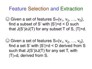
Univariate Dependence • Independence: P(X, Y) = P(X) P(Y) • Measure of dependence: MI(X, Y) = P(X,Y) log dX dY = KL( P(X,Y) || P(X)P(Y) ) P(X,Y) P(X)P(Y)
Other criteria ( chap. 3) A choice of feature selection ranking methods depending on the nature of: • the variables and the target (binary, categorical, continuous) • the problem (dependencies between variables, linear/non-linear relationships between variables and target) • the available data (number of examples and number of variables, noise in data) • the available tabulated statistics.
T-test m- m+ P(Xi|Y=1) P(Xi|Y=-1) -1 xi s- s+ • Normally distributed classes, equal variance s2 unknown; estimated from data as s2within. • Null hypothesis H0: m+ = m- • T statistic: If H0 is true, • t= (m+ - m-)/(swithin1/m++1/m-) Student(m++m--2 d.f.)
Statistical tests ( chap. 2) pval r0 r Null distribution • H0: X and Y are independent. • Relevance index test statistic. • Pvalue false positive rate FPR = nfp / nirr • Multiple testing problem: use Bonferroni correction pval n pval • False discovery rate: FDR = nfp / nscFPRn/nsc • Probe method: FPR nsp/np
Univariate selection may fail Guyon-Elisseeff, JMLR 2004; Springer 2006
Filters,Wrappers, andEmbedded methods Feature subset All features Filter Predictor Multiple Feature subsets All features Predictor Feature subset Embedded method All features Wrapper Predictor
Relief Relief=<Dmiss/Dhit> nearest hit Dhit Dmiss nearest miss Kira and Rendell, 1992 Dhit Dmiss
Wrappers for feature selection Kohavi-John, 1997 N features, 2N possible feature subsets!
Search Strategies ( chap. 4) • Exhaustive search. • Simulated annealing, genetic algorithms. • Beam search: keep k best path at each step. • Greedy search: forward selection or backward elimination. • PTA(l,r): plus l , take away r – at each step, run SFS l times then SBS r times. • Floating search (SFFS and SBFS): One step of SFS (resp. SBS), then SBS (resp. SFS) as long as we find better subsets than those of the same size obtained so far. Any time, if a better subset of the same size was already found, switch abruptly. n-k g
Feature subset assessment m1 m2 m3 N variables/features Split data into 3 sets: training, validation, and test set. 1) For each feature subset, train predictor on training data. 2) Select the feature subset, which performs best on validation data. • Repeat and average if you want to reduce variance (cross-validation). 3) Test on test data. M samples
Single feature relevance Cross validation Relevance in context Embedded Single feature relevance Performance bounds Feature subset relevance Cross validation Single feature relevance Relevance in context Performance learning machine Statistical tests Cross validation Performance bounds Feature subset relevance Nested subset, forward selection/ backward elimination Relevance in context Heuristic or stochastic search Performance bounds Feature subset relevance Performance learning machine Exhaustive search Single feature ranking Statistical tests Wrappers Filters Nested subset, forward selection/ backward elimination Performance learning machine Heuristic or stochastic search Statistical tests Nested subset, forward selection/ backward elimination Exhaustive search Single feature ranking Heuristic or stochastic search Exhaustive search Single feature ranking Three “Ingredients” Assessment Criterion Search
Forward Selection (wrapper) Start n n-1 n-2 1 … Also referred to as SFS: Sequential Forward Selection
Forward Selection (embedded) Start n n-1 n-2 1 … Guided search: we do not consider alternative paths.
Forward Selection with GS Embedded method for the linear least square predictor Stoppiglia, 2002. Gram-Schmidt orthogonalization. • Select a first feature Xν(1)with maximum cosine with the target cos(xi, y)=x.y/||x|| ||y|| • For each remaining feature Xi • Project Xi and the target Y on the null space of the features already selected • Compute the cosine of Xi with the target in the projection • Select the feature Xν(k)with maximum cosine with the target in the projection.
Forward Selection w. Trees At each step, choose the feature that “reduces entropy” most. Work towards “node purity”. All the data f2 f1 Choose f1 Choose f2 • Tree classifiers, like CART (Breiman, 1984)orC4.5 (Quinlan, 1993)
Backward Elimination (wrapper) Also referred to as SBS: Sequential Backward Selection 1 n-2 n-1 n … Start
Backward Elimination (embedded) 1 n-2 n-1 n … Start
Backward Elimination: RFE Embedded method for SVM, kernel methods, neural nets. RFE-SVM, Guyon, Weston, et al, 2002. US patent 7,117,188 • Start with all the features. • Train a learning machine f on the current subset of features by minimizing a risk functional J[f]. • For each (remaining) feature Xi, estimate, without retraining f, the change in J[f] resulting from the removal of Xi. • Remove the feature Xν(k) that results in improving or least degrading J.
Scaling Factors Idea: Transform a discrete space into a continuous space. s=[s1, s2, s3, s4] • Discrete indicators of feature presence:si{0, 1} • Continuous scaling factors:si IR Now we can do gradient descent!
Learning with scaling factors n y ={yj} X={xij} m a s
Formalism ( chap. 5) • Many learning algorithms are cast into a minimization of some regularized functional: Regularization capacity control Empirical error Next few slides: André Elisseeff
Add/Remove features • It can be shown (under some conditions) that the removal of one feature will induce a change in G proportional to: Gradient of f wrt. ith feature at point xk • Examples: SVMs
Recursive Feature Elimination Minimize estimate of R(,) wrt. Minimize the estimate R(,) wrt. and under a constraint that only limited number of features must be selected
Gradient descent • How to minimize? Most approaches use the following method: Would it make sense to perform just a gradient step here too? Gradient step in [0,1]n. Mixes w. many algo. but heavy computations and local minima.
Minimization of a sparsity function • Minimize the number of features used • Replace by another objective function: • l1 norm: • Differentiable function: • Optimize jointly with the primary objective (good prediction of a target).
The l1 SVM • The version of the SVM where ||w||2 is replace by the l1 norm i |wi| can be considered as an embedded method: • Only a limited number of weights will be non zero (tend to remove redundant features) • Difference from the regular SVM where redundant features are all included (non zero weights) Bi et al 2003, Zhu et al, 2003
Mechanical interpretation w2 w2 w* w* w1 w1 J = l ||w||22 + ||w-w*||2 J = ||w||22 + 1/l ||w-w*||2 w2 Lasso w* w1 J = ||w||1+ 1/l ||w-w*||2 Ridge regression Tibshirani, 1996
The l0 SVM • Replace the regularizer ||w||2 by the l0 norm • Further replace by i log( + |wi|) • Boils down to the following multiplicative update algorithm: Weston et al, 2003
Embedded method - summary • Embedded methods are a good inspiration to design new feature selection techniques for your own algorithms: • Find a functional that represents your prior knowledge about what a good model is. • Add the s weights into the functional and make sure it’s either differentiable or you can perform a sensitivity analysis efficiently • Optimize alternatively according to a and s • Use early stopping (validation set) or your own stopping criterion to stop and select the subset of features • Embedded methods are therefore not too far from wrapper techniques and can be extended to multiclass, regression, etc…
Variable/feature selection Y X Remove features Xi to improve (or least degrade) prediction of Y.
What can go wrong? Guyon-Aliferis-Elisseeff, 2007
What can go wrong? X2 Y Y X2 X1 X1 Guyon-Aliferis-Elisseeff, 2007
Causal feature selection Y Y X Uncover causal relationships between Xi and Y.
Tar in lungs Genetic factor2 Bio-marker2 Allergy Systematic noise Biomarker1 Metastasis Coughing Hormonal factor Causal feature relevance Genetic factor1 Smoking Other cancers Anxiety Lung cancer (b)
Formalism:Causal Bayesian networks • Bayesian network: • Graph with random variables X1, X2, …Xn as nodes. • Dependencies represented by edges. • Allow us to compute P(X1, X2, …Xn) as Pi P( Xi | Parents(Xi) ). • Edge directions have no meaning. • Causal Bayesian network: egde directions indicate causality.