Download

1 / 70
740 likes | 1.11k Views
DEMAND THEORY. DR. MOHAMMAD ABDUL MUKHYI, SE.,MM. DEMAND FOR A COMMODITY. Permintaan adalah sejumlah barang yang diminta oleh konsumen pada tingkat harga tertentu.

E N D
DEMAND THEORY DR. MOHAMMAD ABDUL MUKHYI, SE.,MM
DEMAND FOR A COMMODITY Permintaan adalah sejumlah barang yang diminta oleh konsumen pada tingkat harga tertentu. Teori Permintaan adalah menghubungkan antara tingkat harga dengan tingkat kuantitas barang yang diminta pada periode waktu tertentu. Fungsi Permintaan: QdX = ƒ(Px, Py, Pz, I, T, Tech, ….)
Hypothetical Industry Demand Curves for New Domestic Automobiles at Interest Rates of 6%, 8%, and 10%
P P P 2 2 2 1 1 1 d1 d2 d3 0 0 0 3 Q1 Q2 Qx 2 1 2 3 5 Individual 1 Individual 2 Pasar
Permintaan Kentang di Indonesia Permintaan kentang untuk periode 1980-2008: QdS = 7.609 – 1.606PS + 59N + 947I + 479PW + 271t. QdS = quantitas kentang yang dijual per tahun per 1.000 Kg. PS = harga kentang per kg N = rata-rata bergeral jumlah penduduk per 1 milyar. I = pendapatan disposibel per kapita penduduk. PW = harga ubi per kg yang diterima petani. T = trend waktu (t = 1 untuk tahun 1980 dan t = 2 untuk tahun 2008). N = 150,73 I = 1,76PW = 2,94 dan t = 1 Bagaimana bentuk fungsi permintaan kentang?
Elastisitas Harga Permintaan Elastisitas Titik : Elastisitas Busur :
Elastisitas Kumulatif : Elastisitas Silang :
Elastisitas Pendapatan : Elastisitas Harga, Total Revenue, Marginal Revenue : TR = P . Q MR = ΔTR / ΔQ
Q = 600 – 100P Diminta : • Buat fungsi pendapatan. • Hitung nilai pendapatan marginal. • Bila P = 4 dan EP = -2 hitung MR Jawab: • Q = 600 – 100P P = 6 – Q/100 • TR = P.Q TR = (6 – Q/100).Q = 6Q – Q2/100 MR = 6 – Q/50 MR optimal = 0 0 = 6 – Q/50 Q = 300
TR = 6Q – Q2/100 1000 900 TR 800 700 600 TR ($) 500 Q = 600 – 100P 400 300 200 D 100 0 0 200 400 600 800 MR = 6 – Q/50 output
Qx = 1,5 – 3,0Px + 0,8I + 2,0Py – 0,6Ps + 1,2A Qx = penjualan kopi merek X Px = harga kopi merek X I = pendapatan disposibel per kapita per tahun Py = harga kopi pesaing Ps = harga gula per kilo A = pengeluaran iklan untuk kopi merek X Jika Px = 2; I = 2,5; Py = 1,8, Ps = 0.50 dan A = 1 berapa Q? Qx = 1,5 – 3,0(2) + 0,8(2,5) + 2,0(1,8) – 0,6(0,50) + 1,2(1) = 2
Supply Penawaran adalah sejumlah barang yang ditawarkan oleh produsen ke konsumen pada tingkat harga tertentu. Teori Penawaran adalah menghubungkan antara tingkat harga dengan tingkat kuantitas barang yang ditawarkan pada periode waktu tertentu. Fungsi Penawaran: QdX = ƒ(Px, Py, Pz, I, T, Tech, ….)
Hypothetical Industry Supply Curve for New Domestic Automobiles
Hypothetical Industry Supply Curves for New Domestic Automobiles at Interest Rates of 6%, 8%, and 10%
Comparative Statics of Changing Demand and Changing Supply Conditions
Objectives • Understand how regression analysis and other techniques are used to estimate demand relationships • Interpret the results of regression models • economic interpretation • statistical interpretation and tests • Describe special econometric problems of demand estimation
Approaches to Demand Estimation • 1. Surveys, simulated markets, clinics Stated Preference Revealed Preference • 2. Direct Market Experimentation • 3. Regression Analysis
A. Difficulties with Direct Market Experiments (1) expensive and risky (2) never a completely controlled experiment (3) infeasible to try a large number of variations (4) brief duration of experiment
(1) Specify variables: Quantity Demanded, Advertising, Income, Price, Other prices, Quality, Previous period demand, ... (2) Obtain data: Cross sectional v. Time series (3) Specify functional form of equation Linear Yt = a + b X1t + g X2t + ut Multiplicative Yt = a X1tb X2tg et ln Yt = ln a + b ln X1t + g ln X2t + ut (4) Estimate parameters (5) Interpret results: economic and statistical
Violating the assumptions of regression including (1) Multicollinearity- highly correlated independent variables (2) Heteroscedasticity- errors do not have the same variance (3) Serial correlation- error in period t is correlated with error in period t + k (4) Identification problems - data from interaction of supply and demand do not trace out demand relationship
Transit Example • Y P T I H • YEAR Riders Price Pop. Income Parking Rate • 1966 1200 15 1800 2900 50 • 1967 1190 15 1790 3100 50 • 1968 1195 15 1780 3200 60 • 1969 1110 25 1778 3250 60 • 1970 1105 25 1750 3275 60 • 1971 1115 25 1740 3290 70 • 1972 1130 25 1725 4100 75 • 1973 1095 30 1725 4300 75 • 1974 1090 30 1720 4400 75 • 1975 1087 30 1705 4600 80 • 1976 1080 30 1710 4815 80 • 1977 1020 40 1700 5285 80 • 1978 1010 40 1695 5665 85
Y P T I H • YEAR Riders Price Pop. Income Parking Rate • 1979 1010 40 1695 5800 100 • 1980 1005 40 1690 5900 105 • 1981 995 40 1630 5915 105 • 1982 930 75 1640 6325 105 • 1983 915 75 1635 6500 110 • 1984 920 75 1630 6612 125 • 1985 940 75 1620 6883 130 • 1986 950 75 1615 7005 150 • 1987 910 100 1605 7234 155 • 1988 930 100 1590 7500 165 • 1989 933 100 1595 7600 175 • 1990 940 100 1590 7800 175 • 1991 948 100 1600 8000 190 • 1992 955 100 1610 8100 200
Linear Transit Demand Riders = 85.4 – 1.62 price … Pr Elas = -1.62(100/955) in 1992
Multiplicative Transit Demand Ln Riders = exp(3.25)P-.14 …
Ch 3: DEMAND ESTIMATION In planning and in making policy decisions, managers must have some idea about the characteristics of the demand for their product(s) in order to attain the objectives of the firm or even to enable the firm to survive.
Demand information about customer sensitivity to • modifications in price • advertising • packaging • product innovations • economic conditions etc. are needed for product-development strategy • For competitive strategy details about customer reactions to changes in competitor prices and the quality of competing products play a significant role
What Do Customers Want? • How would you try to find out customer behavior? • How can actual demand curves be estimated?
From Theory to Practice D: Qx = f(px, Y, ps, pc, , N) (px=price of good x, Y=income, ps=price of substitute, pc=price of complement, =preferences, N=number of consumers) • What is the true quantitative relationship between demand and the factors that affect it? • How can demand functions be estimated? • How can managers interpret and use these estimations?
Most common methods used are: • consumer interviews or surveys • to estimate the demand for new products • to test customers reactions to changes in the price or advertising • to test commitment for established products b) market studies and experiments • to test new or improved products in controlled settings c) regression analysis • uses historical data to estimate demand functions
Consumer Interviews (Surveys) • Ask potential buyers how much of the commodity they would buy at different prices (or with alternative values for the non-price determinants of demand) • face to face approach • telephone interviews
Consumer Interviews cont’d • Problems: • Selection of a representative sample • what is a good sample? • Response bias • how truthful can they be? • Inability or unwillingness of the respondent to answer accurately
Market Studies and Experiments • More expensive and difficult technique for estimating demand and demand elasticity is the controlled market study or experiment • Displaying the products in several different stores, generally in areas with different characteristics, over a period of time • for instance, changing the price, holding everything else constant
Market Studies and Experimentscont’d • Experiments in laboratory or field • a compromise between market studies and surveys • volunteers are paid to stimulate buying conditions
Market Studies and Experimentscont’d • Problems in conducting market studies and experiments: a) expensive b) availability of subjects c) do subjects relate to the problem, do they take them seriously? BUT: today information on market behavior also collected by membership and award cards
Regression Analysis and Demand Estimation • A frequently used statistical technique in demand estimation • Estimates the quantitative relationship between the dependent variable and independent variable(s) • quantity demanded being the dependent variable • if only one independent variable (predictor) used: simple regression • if several independent variables used: multiple regression
A Linear Regression Model • In practice the dependence of one variable on another might take any number of forms, but an assumption of linear dependency will often provide an adequate approximation to the true relationship
Think of a demand function of general form: Qi = + 1Y - 2 pi + 3ps - 4pc + 5Z + ε where Qi = quantity demanded of good i Y = income pi = price of good i ps = price of substitute(s) pc = price of complement(s) Z = other relevant determinant(s) of demand ε = error term Values of and i ?
and i have to be estimated from historical data • Data used in regression analysis • cross-sectional data provide information on variables for a given period of time • time series data give information about variables over a number of periods of time • New technologies are currently dramatically changing the possibilities of data collection
Simple Linear Regression Model In the simplest case, the dependent variable Y is assumed to have the following relationship with the independent variable X: Y = + X + ε where Y = dependent variable X = independent variable = intercept = slope ε = random factor
Estimating the Regression Equation • Finding a line that “best fits” the data • The line that best fits a collection of X,Y data points, is the line minimizing the sum of the squared distances from the points to the line as measured in the vertical direction • This line is known as a regression line, and the equation is called a regression equation Estimated Regression Line:
Regression with Excel Evaluate statistical significance of regression coefficients using t-test and statistical significance of R2 using F-test
Statistical analysis is testing hypotheses • Statistics is based on testing hypotheses • ”null” hypothesis = ”no effect” • Assume a distribution for the data, calculate the test statistic, and check the probability of getting a larger test statistic value For the normal distribution: Z p
t-test: test of statistical significance of each estimated regression coefficient • i = estimated coefficient • H0: i = 0 • SEβ: standard error of the estimated coefficient • Rule of 2: if absolute value of t is greater than 2, estimated coefficient is significant at the 5% level (= p-value < 0.05) • If coefficient passes t-test, the variable has an impact on demand