Download

1 / 72
1.57k likes | 3.7k Views
Chapter 3 Demand Theory. 1. Consumer Choice and the Law of Demand. Law of Demand. Law of Demand : There is an inverse relationship between the price of a good and the quantity consumers are willing to purchase. As price of a good rises, consumers buy less.

E N D
Law of Demand • Law of Demand: There is an inverse relationship between the price of a good and the quantity consumers are willing to purchase. • As price of a good rises, consumers buy less. • The availability of substitutes --goods that do similar functions -- explains this negative relationship.
Market Demand Schedule • A market demand schedule is a table that shows the quantity of a good people will demand at varying prices. • Consider the market for cellular phones. A market demand schedule lays out the amount of cell phones that are demanded in the market for a spectrum of prices. • We can graph these points (price and the respective demand) to make a demand curve for cell phones.
Jones Smith Two-person market Price Price Price D d d Weekly frozen pizza consumption Individual and Market Demand Curves • Consider Jones’s demand for frozen pizza. At $3.50 Jones demands 1 pizza . . . at $2.50 Jones demands 3 pizzas . . . and so on . . . • Consider Smith’s demand for frozen pizza. At $3.50 Smith demands 2 pizzas . . . at $2.50 Smith demands 3 pizzas . . . and so on . . . • The market demand curve is merely the horizontal sum of the individual demand curves (here Jones and Smith). • The market demand curve will slope downward to the right, just as the individual demand curves do. $3.50 $3.50 $3.50 $2.50 $2.50 $2.50 1 3 2 3 3 6
Demand Market Demand Schedule Price(monthly bill) 140 Millions of Cell Phone Subscribers Cell Phone Price(monthly bill) 120 $123 2.1 100 $107 3.5 $ 92 5.3 80 $ 79 7.6 $ 73 11.0 60 $ 63 16.0 $ 56 24.1 10 15 5 20 25 30 Quantity(of Cell Phone Subscribers)
Demand Market Demand Schedule Price(monthly bill) 140 120 • Notice how the law of demand is reflected by the shape of the demand curve. 100 • As the price of a good rises … 80 • . . . consumers buy less. 60 10 15 5 20 25 30 Quantity(of Cell Phone Subscribers)
Demand Market Demand Schedule Price(monthly bill) 140 120 • The height of the demand curve at any quantity shows the maximum price that consumers are willing to pay for that additional unit. 100 80 • Here, for the 11th unit . . . • . . . consumers are only willing to pay up to $73 for it. 60 • While they would be willing to pay up to $92 for the 5.3 (millionth) unit. 10 15 5 20 25 30 Quantity(of Cell Phone Subscribers)
Consumer Surplus • Consumer Surplus - the area below the demand curve but above the actual price paid. • Consumer surplus is the difference between the amount consumers are willing to pay and the amount they have to pay for a good. • Lower market prices will increase consumer surplus.
MarketPrice = $100 Demand Consumer Surplus Price(monthly bill) • Lets consider the market for cellular phones again. This time we will assume that the demand for cell phones is more linear and that the market price is $100. 140 120 • If the market price is $100, then the 25th unit will not sell because those who demand it are only willing to pay $60 for cellular phone service. 100 80 • At $100, the 15th unit will sell because those who demand it are willing to pay up to $100 for cellular phone service. 60 • At $100, the 10th unit will sell because those who demand it are willing to pay up to $120 for cellular phone service. 10 15 5 20 25 30 Quantity(of Cell Phone Subscribers)
MarketPrice = $100 Demand Consumer Surplus Price(monthly bill) 140 • For all those goods under 15 units, people are willing to pay more than $100 for service. 120 • The area, represented by the distance above the actual price paid and below the demand curve, is called consumer surplus. 100 80 • This area represents the net gains to buyers from market exchange. 60 10 15 5 20 25 30 Quantity(of Cell Phone Subscribers)
Changes in Demand and Quantity Demanded • Change in Demand - shift in entire demand curve. • Change in Quantity Demanded - movement along the same demand curve in response to a price change.
D2 Change in Demand Price(dollars) 25 • If CDs cost $15 each, the CD demand curve D1 shows that 10 units would be demanded. 20 • If the price of CDs changed to $7.50, the quantity demanded for CDs would increase to 20 units. 15 • If, somehow, the preferences for CDs changed then the demandfor CDs may change. 10 5 • Here we will assume that consumer income increases, increasing demand for CDs at all price levels. At $15 15 units are now demanded. D1 10 15 5 10 15 20 20 25 30 Quantity(of Compact Disks per yr)
Demand Curve Shifters • Changes in Consumer Income • Change in the Number of Consumers • Change in Price of Related Good • Changes in Expectations • Demographic Changes • Changes in Consumer Tastes and Preferences
1. Which of the following do you think would lead to an increase in the current demand for beef: (a) higher pork prices, (b) higher incomes, (c) higher prices of grains used to feed cows, (d) good weather conditions leading to a bumper (very good) corn crop, (e) an increase in the price of beef? Questions for Thought: 2. What is being held constant when a demand curve for a specific product (like shoes or apples, for example) is constructed? Explain why the demand curve for a product slopes downward and to the right.
The Market Demand Curve Shows the total quantity of the good that would be purchased at each price
Other Determinants of Market Demand • Consumer tastes and preferences. • Consumer incomes. • Level of other prices. • Size of consumer population.
Demand Functions Q of good X = f ( Price of X, Incomes of consumers, Prices of other goods, Population, Advertising expenditures, Etc.)
Elastic and Inelastic Demand Curves • Elastic demand - quantity demanded is sensitive to small price changes. • Easy to substitute away from good. • Inelastic demand - quantity demanded is not sensitive to price changes. • Difficult to substitute away from good.
Elastic and Inelastic Demand Curves • If the market price for gasoline was to rise from $1.25 to $2.00, the quantity demanded in the market decreases insignificantly (from 8 to 7 units). 2.00 Gasoline 1.25 • If the market price for tacos rises from $1.25 to $2.00, the quantity demanded in the market decreases significantly (from 8 to 1 unit). 6 10 2 4 5 7 9 1 3 8 2.00 Tacos • Taco demand is highly sensitive to price changes and can be described as elastic; gasoline demand is relatively insensitive to price changes and can be described as inelastic. 1.25 6 10 2 4 5 7 9 1 3 8
% Change in quantity demanded % Q Price Elasticityof demand % P % Change in Price Elasticity of Demand • Price elasticity reveals the responsiveness of the amount purchased to a change in price. = = - or put simply -
Price Price Price Mythicaldemandcurve • Perfectly inelastic: Despite an increase in price, consumers still purchase the same amount. In fact, the substitution and income effects prevent this from happening in the real world. Quantity/time Quantity/time Quantity/time Demandfor Cigarettes (a) • Relatively inelastic: A percent increase in price results in a smaller % reduction in sales. The demand for cigarettes has been estimated to be highly inelastic. (b) Demand curve of unitary elasticity • Unitary elasticity: The % change in quantity demanded is equal to the % change in price. A curve of decreasing slope results. Sales revenue (price times quantity sold) is constant. (c) Elasticity of Demand
Price Price • Relatively elastic: A percent increase in price leads to a larger % reduction in purchases. When good substitutes are available for a product (as is the case for apples), the amount purchased will be highly sensitive to a change in price. Quantity/time Quantity/time (d) Demandfor Apples • Perfectly elastic: Consumers will buy all of Farmer Jones’s wheat at the market price, but none will be sold above the market price. Demand for Farmer Jones’s wheat (e) Elasticity of Demand
Recall - = Elasticity (– ) 0.14 ( - ) 0.14 = D Elasticity of Demand (110 - 100) (110 + 100) Price($) ($1 - $2) ($1 + $2) • With this straight-line (constant-slope) demand curve, demand varies across a range of prices. • Using the equation for elasticity from before, the formula for arc elasticity shows that, when price rises from $1 to $2 . . . and quantity demanded falls from 110 to 100 . . . the elasticity for that region of the demand curve is ( - .14 ) (inelastic). 2 1 100 110 QuantityDemanded /Time
Recall - = Elasticity (– ) 7.0 ( - ) 7.0 = D Elasticity of Demand (20 - 10) (20 + 10) Price($) ($10 - $11) ($10 + $11) • A price increase of the same magnitude (but a smaller %) from $10 to $11 . . . 11 leads to a decline in quantity demanded from 20 to 10. Even though the change in price here was smaller than before (as a %) the same change in quantity demanded occurred. 10 • Using the same equation to calculate elasticity as before, the elasticity amounts to - 7.0 (greater than - .14 from before). • Thus the price-elasticity of a straight-line demand curve increases as price rises. 10 20 QuantityDemanded /Time
Determinants of Price Elasticity of Demand • Availability of substitutes • When good substitutes for a product are available, a rise in price induces many consumers to switch to other products causing demand to be elastic. • Share of total budget expended on product • As the share of the total budget expended on the product rises, demand is more elastic.
Elastic and Inelastic Demand Price Price $1.50 $1.50 $1.00 $1.00 D D 25 100 90 100 (a) Ballpoint pens per week (in thousands) (b) Cigarette packs per week (in millions) • As the price of ballpoint pens (a) rises from $1.00 to $1.50 (a 50% increase in price). . . quantity demanded plunges from 100,000 to 25,000 (a 75% decrease in quantity demanded). • The % reduction in quantity demanded is larger than the % increase in price, thus the demandfor ballpoint pens is elastic. • As the price of cigarettes (b) rises from $1.00 to $1.50 (a 50% increase in price). . . quantity demanded plunges from 100 mil. to 90 mil. (a 10% decrease in quantity demanded). • The % reduction in quantity demanded is smaller than the % increase in price, thus the demandfor cigarettes is inelastic.
Time and Demand Elasticity • If the price of a product increases, consumers will reduce their consumption by a larger amount in the long run than in the short run. • Thus, the demand for most products will be more elastic in the long run than in the short run. • This relationship is often referred to as the second law of demand.
Elasticity of Demand APPROXIMATELY UNITARY ELASTICITY INELASTIC Movies 0.9 Salt 0.1 Housing, owner occupied (long run) 1.2 Matches 0.1 Shellfish (consumed at home) 0.9 Oysters (consumed at home) 1.1 Toothpicks 0.1 Private education 1.1 Airline travel (short run) 0.1 Tires (short run 0.9 Gasoline (short run) 0.2 Tires (long run) 1.2 Gasoline (long run) 0.7 Radio and television receivers 1.2 Residential natural gas (short run) 0.1 Residential natural gas (long run) 0.5 Coffee 0.25 Fish (cod), consumed at home 0.5 ELASTIC Tobacco products (short run) 0.45 Restaurant meals 2.3 Legal services (short run) 0.4 Foreign travel (long run) 4.0 Physician services 0.6 Airline travel (long run) 2.4 Taxi (short run) 0.6 Fresh green peas 2.8 Automobiles (long run) 0.2 Automobiles (short run 1.2–1.5 Chevrolet automobiles 4.0 Fresh tomatoes 4.6 • Can you explain why the demand for some goods is highly inelastic while that for others is elastic.
Price elasticity of demand The percentage change in quantity demanded resulting from a 1 percent change in price. h = - dQ xP dP Q
Arc elasticities uses average values of Q and P as reference points h = - dQ x(P1 + P2)/2 dP (Q1 + Q2)/2
5. Total Revenue, Total Expenditure, and the Price Elasticity of Demand
-- unchanged -- unchanged -- -- Total Expenditures and Demand Elasticity Impact of Lowering Priceon Total ConsumerExpenditures or a Firm’sTotal Revenue Impact of Raising Price on Total Consumer Expenditures or a Firm’sTotal Revenue NumericalElasticityCoefficient(In Absolute Value) Price ElasticityOf Demand 1 to Elastic decrease increase Unitary Elastic 1 Inelastic 0 to 1 increase decrease • The table above summarizes the relationship between changes in price and total expenditures for demand curves of varying elasticity.
(b) The Firm’s Demand Curve, Total Revenue, and Elasticity Price Price Elasticity Here demand is elastic so lower prices result in more e = 17.00 revenue and higher prices $9 e = 5.00 result in less revenue $8 e = 2.60 Total revenue unchanged $7 by price when demand is e = 1.57 $6 unitary elastic e = 1.00 $5 Here demand is inelastic e = 0.64 $4 so lower prices result in e = 0.38 less revenue and higher $3 prices result in more e = 0.20 $2 revenue e = 0.06 $1 (a) The Firm’s Price, Quantity Sold, Total Revenue, and Price Elasticity $0 Quantity 0 1 2 3 4 5 6 7 8 9 Quantity Total Price Sold Revenue Price Elasticity of Demand x = $9 0 $0 x = $8 1 $8 x = $7 2 $14 x = $6 3 $18 x = $5 4 $20 x = $4 5 $20 x = $3 6 $18 x = $2 7 $14 x = $1 8 $8 x = $0 9 $0 Total Revenues and Demand Elasticity P XQ = TR $9 x 0 = $0 $8 x 1 = $8 $7 x 2 = $14 $6 x 3 = $18 $5 x 4 = $20 $4 x 5 = $20 $3 x 6 = $18 $2 x 7 = $14 $1 x 8 = $8 $0 x 9 = $0 ((0-1) / (0+1)) / ((9-8) / (9+8)) = 17.00 • By tracing out the demand curve, one can follow how changes in price (through changes in quantity demanded) change total revenue collected. ((1-2) / (1+2)) / ((8-7) / (8+7)) = 5.00 ((2-3) / (2+3)) / ((7-6) / (7+6)) = 2.60 ((3-4) / (3+4)) / ((6-5) / (6+5)) = 1.57 ((4-5) / (4+5)) / ((5-4) / (5+4)) = 1.00 • By calculating the price elasticity of demand at different points along the demand curve, one can follow how and where total revenue is maximized. ((5-6) / (5+6)) / ((4-3) / (4+3)) = 0.64 ((6-7) / (6+7)) / ((3-2) / (3+2)) = 0.38 ((7-8) / (7+8)) / ((2-1) / (2+1)) = 0.20 ((8-9) / (8+9)) / ((1-0) / (1+0)) = 0.06
Total Revenue ismaximized somewherebetween $4 and $5 (where demand isunitary elastic). Total Revenue ismaximized somewherebetween 4 and 5 units (again, where demand is unitary elastic). Price Total Revenue $9 $20 $8 $7 $15 $6 $5 $10 $4 $3 $5 $2 $1 $0 $0 0 1 2 3 4 5 6 7 8 9 $0 $5 $10 $15 $20 Quantity Total Revenue (d) Quantity versus Total Revenue (c) Price versus Total Revenue Total Revenues and Demand Elasticity • The firm maximizes its revenue at the price (or quantity) where demand is unitary elastic. (a) The Firm’s Price, Quantity Sold, & Total Revenue Quantity Total Elasticity Price Sold Revenue x = $9 0 $0 17.00 x = $8 1 $8 5.00 x = $7 2 $14 2.60 x = $6 3 $18 1.57 x = $5 4 $20 1.00 x = $4 5 $20 .64 x = $3 6 $18 .38 x = $2 7 $14 .20 x = $1 8 $8 .06 x = $0 9 $0
Price Elasticity of Demand and Total Expenditures • h> 1 ==> an inverse relationship between price changes and total expenditures. • h< 1 ==> a direct relationship between price changes and total expenditures. • h= 1 ==> no change in total expenditures as price changes.
Total Revenue, Marginal Revenue, and Price Elasticity Suppose P = a - bQ, then TR = aQ - bQ2 MR = dTR/dQ = a - 2bQ Since h = -(dQ/dP) x (P/Q) h = 1/b x (a - bQ)/Q
Price a h > 1 Demand and MR h = 1 h < 1 Quantity a/2b a/b Dollars Total Revenue Quantity
Marginal Revenue, Price and Price Elasticity MR = P [ 1 - (1/h)]
Determinants of Price Elasticity of Demand Elasticity is greater when: • there are more substitutes for the product. • the product is a more important part of a consumer’s budget. • the time period under consideration is greater.
Income Elasticityof demand % Change in quantity demanded % Change in Income Income Elasticity • Income elasticityindicates the responsiveness of the demand for a product to a change in income. =
Income Elasticity of Demand • Income Elasticity of Demand: This is measure of the responsiveness of the demand for a good to changes in consumer income. It is measured by the percentage change in quantity demanded divided by the percentage change in buyer income • Normal Good: Positive income elasticity • Inferior Good: Negative income elasticity
Income Elasticity • A normal good is any good with a positive income elasticity of demand. • As income expands, the demand for normal goods will rise. • Goods with a negative income elasticity are inferior goods. • As income expands, the demand for inferior goods will decline.
Income Elasticity The percentage change in quantity demanded resulting from a 1 percent change in consumer income h I =dQ xI dI Q
Cross Price Elasticity of Demand • Cross Price Elasticity of Demand: This is a measure of the responsiveness of the demand for a good to changes in the price of a related good. It is measured by the percentage change in the quantity demanded one one good (say, Coke) divided by the percentage change in the price of a related good (say, Pepsi) C = {QX/QX}/{PY/PY}
Cross Elasticity The percentage change in quantity demanded of good X resulting from a 1 percent change in the price of good Y hX,Y=dQxxPY dPy Qx