Download
1 / 28
280 likes | 411 Views
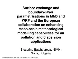
Surface exchange and boundary-layer parametrisations in MM5 and WRF and the European collaboration on enhancing meso-scale meteorological modelling capabilities for air pollution and dispersion applications Ekaterina Batchvarova, NIMH, Sofia, Bulgaria. OUTLINE: The ABL

E N D
Surface exchange and boundary-layer parametrisations in MM5 and WRF and the European collaboration on enhancing meso-scale meteorological modelling capabilities for air pollution and dispersion applications Ekaterina Batchvarova, NIMH, Sofia, Bulgaria
OUTLINE: The ABL Limits of applicability of the parameterisations used in mesoscale models: urban areas aggregation within a grid cell in nonhonogeneous areas stable conditions very low wind speeds
Two-way coupling WRF/CFD through MCEL (Model Coupling Environmental Library)Fei Chen et al, Integrated Urban Modeling System for the Community WRF Model: Current Status and Future Plan,Workshop on Model Urbanization Strategy, Exeter, UK. 3-4 May 2007 CFD-Urban: Hi-Res Urban Model WRF-Noah/UCM coupled model forecast Coupling Down-Scale Up- Scale CFD-Urban: T&D
The height of the atmospheric boundary layer (ABL)
Top of mixing layer Top of mixing layer
The urban boundary-layer height Florence Berlin
COST 728 Action “Enhancing Meso-Scale Meteorological Modelling Capabilities For Air Pollution And Dispersion Applications” COST Action 732 “Quality Assurance and Improvement of Micro-Scale Meteorological Models”
Why is the ABL height important? Scaling parametre for the wind profile (wind energy as example) Scaling parameter for turbulence (wind turbine load and design, dispersion of air pollution) Acts as a lid for air pollution (air pollution concentration, atmospheric chemistry) Influences the formation of clouds and ship trails Influences propagation of radar and microwave signals and many more……
Wind profiles over flat terrain U:Urban R:residential measurements 250 meter tall mastin Hamburg, Germany
The ABL height influences the wind profile above 50 m (above the surface layer) without ABL height with ABL height
What is it and how does it look? Schematic structure of the growing convective boundary layer. The surface in this case is more humid than the free atmosphere which is typical for vegetated areas.
Model for the mixed-layer height The derivation is based on the equation for heat conservation and the budget equation for turbulent kinetic energy: Heat conservation: Heat flux at the top of the mixed layer: Strength of the inversion: Heating rate of the mixed layer: , Idealized (zero-order model) of the mixed-layer
Turbulent kinetic energy budget: Parameterized budget for turbulent kinetic energy: where lhs represent consumption of potential and kinetic energy by the entrainment process the rhs represents production of turbulent kinetic turbulent energy by heat flux and wind shear Solving for the heat flux at the inversion reads: , Batchvarova and Gryning, 1991: BLM
It is possible to derive an analytical solution for , but it is unattractive for applied use. An approximation to the analytical solution is suggested with the correct asymptotic limits for neutral and convective conditions Solid line the analytical solution, dashed line its approximation
Applying these expressions and the approximation for Δ a differential equation for the height of the internal boundary layer, h, can be derived: III I II The spin-up term (III) dominates the growth of the shallow boundary layer Further growth makes the contribution of of mechanical turbulence (II) increasingly important until the boundary layer reaches a height of about -1.4L, where convective turbulence (I) takes over the control of the growth process. Batchvarova and Gryning, 1991: BLM
Coastal area – Internal Boundary Layer Gryning and Batchvarova, 1990: QJRMS
Model for the entrainment zone And First order ABL model Entrainment Richardson number: Entrainment zone depth: When the ABL is growing fast, (morning) the entrainment zone can be 60% of it. Later in the day it becomes smaller, empirical limit is 20% of the ABL height The entrainment zone depth estimated from Sodar measurements close to Berlin, Germany. The dashed line represent the parameterisation suggested by Gryning and Batchvarova (1994). The figures indicate the number of cases in each class, and the error bars the standard deviation.
Simulations of the height of the internal boundary layer over land The Vancouver cases
Tethersonde measurements and model simulations of the mixing height in Central Vancouver (Sunset site)
Pacific-93 Air-plane measurements by a downlooking lidar. Flight legs (full lines), there are 3 legs Intensive network (filled circles) of wind measurements Dashed line, model simulations Full line lidar measurements
Modelled and measured marine boundary layer height Christiansø Radiosoundings
Mixing height estimated by the HIRLAM model (weather prediction) The critical Richardson number method: Sørensen (1998) Vogelezang and Holtslag (1996) . Boundary-layer heights over Christiansø during the extensive observation period, estimated from profiles of wind and temperature from the HIRLAM model, are shown by thin lines. The left panel shows the results using the Richardson number suggested by Sørensen, the right panel when using the Richardson number in Vogelezang and Holtslag. Bullets show the measurements. The thick line illustrates a running mean over 9 points.
The urban boundary layer on top: ABL height then: the blended layer red: internal boundary layer green: inertial sublayer blue: roughness sublayer Highly simplified
The height of the roughess sublayer Under convective conditions, Above the roughness sublayer in urban areas similarity theory and dispersion models are valid – hence the Mesoscale Meteorological and Air Pollution Models are applicable. If the first sigma-level is high enough, it can be used. The 2 m and 10 m values (derived via MO Similarity relations) from the first model level are not true. The level of 40 m is within the inertial sublayer
Different measurement techniques register different parameters, hence correspond to different definitions of ABL (inversion in pot. Temperature is derived from radiosoundings, cloud base is detected by ceilometers, layers of accumulated aerosols are detected by sodars and lidars
Two-way coupling WRF/CFD through MCEL (Model Coupling Environmental Library)Fei Chen et al, Integrated Urban Modeling System for the Community WRF Model: Current Status and Future Plan,Workshop on Model Urbanization Strategy, Exeter, UK. 3-4 May 2007 CFD-Urban: Hi-Res Urban Model WRF-Noah/UCM coupled model forecast Coupling Down-Scale Up- Scale CFD-Urban: T&D