Download
1 / 11
570 likes | 1.67k Views
Correlation. A correlation exists between two variables when one of them is related to the other in some way. A scatterplot is a graph in which the paired ( x,y ) sample data are plotted on a graph.

E N D
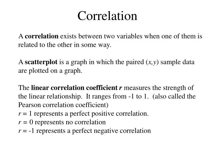
Correlation A correlation exists between two variables when one of them is related to the other in some way. A scatterplot is a graph in which the paired (x,y) sample data are plotted on a graph. The linear correlation coefficientr measures the strength of the linear relationship. It ranges from -1 to 1. (also called the Pearson correlation coefficient) r = 1 represents a perfect positive correlation. r = 0 represents no correlation r = -1 represents a perfect negative correlation
Perfect positive Strong positive Positive correlation r = 1 correlation r = 0.99 correlation r = 0.80 Strong negative No Correlation Non-linear correlation r = -0.98 r = 0.16 relationship
Meanings r2 represents the proportion of the variation in y that is explained by the linear relationship between x and y. Example: Using the heights and weights for a group of models, you find the correlation coefficient to be r = 0.796. r2 = 0.634. We conclude that about 63.4% of the models’ weight can be explained by the relationship between height and weight. This suggests that 36.6% of the variation in weights cannot be explained by height.
Hypothesis Test for Correlation where ρ (rho) is the population correlation coefficient Be careful not to confuse ρ with p Use Table A-6 in pullout to find critical values for r. Example: For the group of models, we had r=0.796. This was based on a sample size of 9. Using a significance level of 0.05, we find the critical value is 0.666. Since our r is larger than the critical value, we reject the null hypothesis, and conclude that there is a significant correlation
Big issues to be aware of: 1. Correlation does not imply causation. For example, there is a strong correlation between golf scores and salaries for CEOs. This does not imply (as one reporter suggested) that one can improve their salary by getting better at golf. Often times there are lurking variables, which is something that affects both variables being studied, but is not included in the study. 2. Beware data based on averages. Averages suppress individual variation, and can artificially inflate the correlation coefficient. 3. Look out for non-linear relationships. Just because there is no linear correlation does not mean that the variables might not be related in another way.
Regression If there is a relationship between x and y, we might want to find the equation of a line that best approximates the data. This is called the regression line (also called best-fit line or least-squares regression line). We can use this line to make predictions.
Example There is a positive correlation between the circumference of a tree and its height (r = 0.828). The regression line has equation We could use this equation to estimate the height of a tree with circumference 4ft:
Tree graph Note: Outliers can strongly influence the graph of the regression line and inflate the correlation coefficient. In the above example, removing the outlier drops the correlation coefficient from r = 0.828 to r = 0.678.
Finding the correlation coefficient and regression equation How not to do it: Instead: Use technology! Our calculators can do it, as can Excel and various other statistical packages.
y=ax+b a=.6403301887 b=22.87712264 r2=.55158844554 r=.7426900063 Is there a significant relationship? Predict a female child’s height if the mother’s height is 62 inches
HW 9.2: 1, 3, 9, 11 HW 9.3: 1, 3, 9, 11 9 11 y=ax+b a=-.0111 b=6.76 r2=.013924 r=-.118 y=ax+b a=.769 b=-14.4 r2=.432964 r=.658