Download
1 / 95
1.22k likes | 2.23k Views
Radio Propagation - Large-Scale Path Loss. CS 515 Mobile and Wireless Networking Ibrahim Korpeoglu Computer Engineering Department Bilkent University, Ankara. Reading Homework Due Date: Next Wednesday. Read the handouts that wa have put into the library Read the following paper:

E N D
Radio Propagation - Large-Scale Path Loss CS 515 Mobile and Wireless Networking Ibrahim Korpeoglu Computer Engineering Department Bilkent University, Ankara
Reading HomeworkDue Date: Next Wednesday • Read the handouts that wa have put into the library • Read the following paper: • J. B. Andersen, T. S. Rappaport, S. Yoshida, Propagation Measurements and Models for Wireless Communications Channels, IEEE Communications Magazine, (January 1995), pp. 42-49. • Read Chapter 4 of Rappaport’s Book. • You have of course read the previous 4 papers! Ibrahim Korpeoglu
Basics • When electrons move, they create electromagnetic waves that can propagate through the space • Number of oscillations per second of an electromagnetic wave is called its frequency, f, measured in Hertz. • The distance between two consecutive maxima is called the wavelength, designated by l. Ibrahim Korpeoglu
Basics • By attaching an antenna of the appropriate size to an electrical circuit, the electromagnetic waves can be broadcast efficiently and received by a receiver some distance away. • In vacuum, all electromagnetic waves travel at the speed of light: c = 3x10⁸ m/sec. • In copper or fiber the speed slows down to about 2/3 of this value. • Relation between f, l , c: lf = c Ibrahim Korpeoglu
Basics • We have seen earlier the electromagnetic spectrum. • The radio, microwave, infrared, and visible light portions of the spectrum can all be used to transmit information • By modulating the amplitude, frequency, or phase of the waves. Ibrahim Korpeoglu
Basics • We have seen wireless channel concept earlier: it is characterized by a frequency band (called its bandwidth) • The amount of information a wireless channel can carry is related to its bandwidth • Most wireless transmission use narrow frequency band (Df << f) • Df: frequency band • f: middle frequency where transmission occurs • New technologies use spread spectrum techniques • A wider frequency band is used for transmission Ibrahim Korpeoglu
Basics - Propagation • Radio waves are • Easy to generate • Can travel long distances • Can penetrate buildings • They are both used for indoor and outdoor communication • They are omni-directional: can travel in all directions • They can be narrowly focused at high frequencies (greater than 100MHz) using parabolic antennas (like satellite dishes) • Properties of radio waves are frequency dependent • At low frequencies, they pass through obstacles well, but the power falls off sharply with distance from source • At high frequencies, they tend to travel in straight lines and bounce of obstacles (they can also be absorbed by rain) • They are subject to interference from other radio wave sources Ibrahim Korpeoglu
Basics - Propagation At VLF, LF, and MF bands, radio waves follow the ground. AM radio broadcasting uses MF band reflection At HF bands, the ground waves tend to be absorbed by the earth. The waves that reach ionosphere (100-500km above earth surface), are refracted and sent back to earth. Ionosphere absorption Ibrahim Korpeoglu
Basics - Propagation VHF Transmission LOS path Reflected Wave • Directional antennas are used • Waves follow more direct paths • - LOS: Line-of-Sight Communication • - Reflected wave interfere with the original signal Ibrahim Korpeoglu
Basics - Propagation • Waves behave more like light at higher frequencies • Difficulty in passing obstacles • More direct paths • They behave more like radio at lower frequencies • Can pass obstacles Ibrahim Korpeoglu
Propagation Models • We are interested in propagation characteristics and models for waves with frequencyy in range: few MHz to a few GHz • Modeling radio channel is important for: • Determining the coverage area of a transmitter • Determine the transmitter power requirement • Determine the battery lifetime • Finding modulation and coding schemes to improve the channel quality • Determine the maximum channel capacity Ibrahim Korpeoglu
Radio Propagation Models • Transmission path between sender and receiver could be • Line-of-Sight (LOS) • Obstructed by buildings, mountains and foliage • Even speed of motion effects the fading characteristics of the channel Ibrahim Korpeoglu
Radio Propagation Mechanisms • The physical mechanisms that govern radio propagation are complex and diverse, but generally attributed to the following three factors • Reflection • Diffraction • Scattering • Reflection • Occurs when waves impinges upon an obstruction that is much larger in size compared to the wavelength of the signal • Example: reflections from earth and buildings • These reflections may interfere with the original signal constructively or destructively Ibrahim Korpeoglu
Radio Propagation Mechanisms • Diffraction • Occurs when the radio path between sender and receiver is obstructed by an impenetrable body and by a surface with sharp irregularities (edges) • Explains how radio signals can travel urban and rural environments without a line-of-sight path • Scattering • Occurs when the radio channel contains objects whose sizes are on the order of the wavelength or less of the propagating wave and also when the number of obstacles are quite large. • They are produced by small objects, rough surfaces and other irregularities on the channel • Follows same principles with diffraction • Causes the transmitter energy to be radiated in many directions • Lamp posts and street signs may cause scattering Ibrahim Korpeoglu
Radio Propagation Mechanisms R transmitter Street S D D Building Blocks R: Reflection D: Diffraction S: Scattering receiver Ibrahim Korpeoglu
Radio Propagation Mechanisms • As a mobile moves through a coverage area, these 3 mechanisms have an impact on the instantaneous received signal strength. • If a mobile does have a clear line of sight path to the base-station, than diffraction and scattering will not dominate the propagation. • If a mobile is at a street level without LOS, then diffraction and scattering will probably dominate the propagation. Ibrahim Korpeoglu
Radio Propagation Models • As the mobile moves over small distances, the instantaneous received signal will fluctuate rapidly giving rise to small-scale fading • The reason is that the signal is the sum of many contributors coming from different directions and since the phases of these signals are random, the sum behave like a noise (Rayleigh fading). • In small scale fading, the received signal power may change as much as 3 or 4 orders of magnitude (30dB or 40dB), when the receiver is only moved a fraction of the wavelength. Ibrahim Korpeoglu
Radio Propagation Models • As the mobile moves away from the transmitter over larger distances, the local average received signal will gradually decrease. This is called large-scale path loss. • Typically the local average received power is computed by averaging signal measurements over a measurement track of 5l to 40l. (For PCS, this means 1m-10m track) • The models that predict the mean signal strength for an arbitrary-receiver transmitter (T-R) separation distance are called large-scale propagation models • Useful for estimating the coverage area of transmitters Ibrahim Korpeoglu
Small-Scale and Large-Scale Fading Received Power (dBm) -30 -40 -50 -60 This figure is just an illustrationto show the concept. It is not based on read data. -70 14 16 18 20 22 24 26 28 T-R Separation (meters) Ibrahim Korpeoglu
What is Decibel (dB) • What is dB (decibel): • A logarithmic unit that is used to describe a ratio. • Let say we have two values P1 and P2. The difference (ratio) between them can be expressed in dB and is computed as follows: • 10 log (P1/P2) dB • Example: transmit power P1 = 100W, received power P2 = 1 W • The difference is 10log(100/1) = 20dB. Ibrahim Korpeoglu
dB • dB unit can describe very big ratios with numbers of modest size. • See some examples: • Tx power = 100W, Received power = 1W • Tx power is 100 times of received power • Difference is 20dB • Tx power = 100W, Received power = 1mW • Tx power is 100,000 times of received power • Difference is 50dB • Tx power = 1000W, Received power = 1mW • Tx power is million times of received power • Difference is 60dB Ibrahim Korpeoglu
dBm • For power differences, dBm is used to denote a power level with respect to 1mW as the reference power level. • Let say Tx power of a system is 100W. • Question: What is the Tx power in unit of dBm? • Answer: • Tx_power(dBm) = 10log(100W/1mW) = 10log(100W/0.001W) = 10log(100,0000) = 50dBm Ibrahim Korpeoglu
dBW • For power differences, dBW is used to denote a power level with respect to 1W as the reference power level. • Let say Tx power of a system is 100W. • Question: What is the Tx power in unit of dBW? • Answer: • Tx_power(dBW) = 10log(100W/1W) = 10log(100) = 20dBW. Ibrahim Korpeoglu
Decibel (dB) versus Power Ratio Comparison of two Sound Systems Ibrahim Korpeoglu
Free-Space Propagation Model • Used to predict the received signal strength when transmitter and receiver have clear, unobstructed LOS path between them. • The received power decays as a function of T-R separation distance raised to some power. • Path Loss: Signal attenuation as a positive quantity measured in dB and defined as the difference (in dB) between the effective transmitter power and received power. Ibrahim Korpeoglu
Free-Space Propagation Model • Free space power received by a receiver antenna separated from a radiating transmitter antenna by a distance d is given by Friis free space equation: Pr(d) = (PtGtGrl2) / ((4p)2d2L) [Equation 1] • Pt is transmited power • Pr(d) is the received power • Gt is the trasmitter antenna gain (dimensionless quantity) • Gr is the receiver antenna gain (dimensionless quantity) • d is T-R separation distance in meters • L is system loss factor not related to propagation (L >= 1) • L = 1 indicates no loss in system hardware (for our purposes we will take L = 1, so we will igonore it in our calculations). • l is wavelength in meters. Ibrahim Korpeoglu
Free-Space Propagation Model • The gain of an antenna G is related to its affective aperture Ae by: • G = 4pAe / l2 [Equation 2] • The effective aperture of Ae is related to the physical size of the antenna, • l is related to the carrier frequency by: • l = c/f = 2pc / wc [Equation 3] • f is carrier frequency in Hertz • wc is carrier frequency in radians per second. • c is speed of light in meters/sec Ibrahim Korpeoglu
Free-Space Propagation Model • An isotropic radiator is an ideal antenna that radiates power with unit gain uniformly in all directions. It is as the reference antenna in wireless systems. • The effective isotropic radiated power (EIRP) is defined as: • EIRP = PtGt[Equation 4] • Antenna gains are given in units of dBi (dB gain with respect to an isotropic antenna) or units of dBd (dB gain with respect to a half-wave dipole antenna). • Unity gain means: • G is 1 or 0dBi Ibrahim Korpeoglu
Free-Space Propagation Model • Path loss, which represents signal attenuation as positive quantity measured in dB, is defined as the difference (in dB) between the effective transmitted power and the received power. PL(dB) = 10 log (Pt/Pr) = -10log[(GtGrl2)/(4p)2d2] [Equation 5] (You can drive this from equation 1) • If antennas have unity gains (exclude them) PL(dB) = 10 log (Pt/Pr) = -10log[l2/(4p)2d2] [Equation 6] Ibrahim Korpeoglu
Free-Space Propagation Model • For Friis equation to hold, distance d should be in the far-field of the transmitting antenna. • The far-field, or Fraunhofer region, of a transmitting antenna is defined as the region beyond the far-field distance df given by: • df = 2D2/l [Equation 7] • D is the largest physical dimension of the antenna. • Additionally, df >> D and df >> l Ibrahim Korpeoglu
Free-Space Propagation Model – Reference Distance d0 • It is clear the Equation 1 does not hold for d = 0. • For this reason, models use a close-in distance d0 as the receiver power reference point. • d0 should be >= df • d0 should be smaller than any practical distance a mobile system uses • Received power Pr(d), at a distance d > d0 from a transmitter, is related to Pr at d0, which is expressed as Pr(d0). • The power received in free space at a distance greater than d0 is given by: Pr(d) = Pr(d0)(d0/d)2 d >= d0 >= df [Equation 8] Ibrahim Korpeoglu
Free-Space Propagation Model • Expressing the received power in dBm and dBW • Pr(d) (dBm) = 10 log [Pr(d0)/0.001W] + 20log(d0/d)where d >= d0 >= df and Pr(d0) is in units of watts. [Equation 9] • Pr(d) (dBW) = 10 log [Pr(d0)/1W] + 20log(d0/d)where d >= d0 >= df and Pr(d0) is in units of watts.[Equation 10] • Reference distance d0 for practical systems: • For frequncies in the range 1-2 GHz • 1 m in indoor environments • 100m-1km in outdoor environments Ibrahim Korpeoglu
Example Question • A transmitter produces 50W of power. • A) Express the transmit power in dBm • B) Express the transmit power in dBW • C) If d0 is 100m and the received power at that distance is 0.0035mW, then find the received power level at a distance of 10km. • Assume that the transmit and receive antennas have unity gains. Ibrahim Korpeoglu
Solution • A) • Pt(W) is 50W. • Pt(dBm) = 10log[Pt(mW)/1mW)]Pt(dBm) = 10log(50x1000)Pt(dBm) = 47 dBm • B) • Pt(dBW) = 10log[Pt(W)/1W)]Pt(dBW) = 10log(50)Pt(dBW) = 17 dBW Ibrahim Korpeoglu
Solution • Pr(d) = Pr(d0)(d0/d)2 • Substitute the values into the equation: • Pr(10km) = Pr(100m)(100m/10km)2Pr(10km) = 0.0035mW(10-4)Pr(10km) = 3.5x10⁻¹⁰W • Pr(10km) [dBm] = 10log(3.5x10⁻¹⁰W/1mW) = 10log(3.5x10⁻⁷) = -64.5dBm Ibrahim Korpeoglu
Two main channel design issues • Communication engineers are generally concerned with two main radio channel issues: • Link Budged Design • Link budget design determines fundamental quantities such as transmit power requirements, coverage areas, and battery life • It is determined by the amount of received power that may be expected at a particular distance or location from a transmitter • Time dispersion • It arises because of multi-path propagation where replicas of the transmitted signal reach the receiver with different propagation delays due to the propagation mechanisms that are described earlier. • Time dispersion nature of the channel determines the maximum data rate that may be transmitted without using equalization. Ibrahim Korpeoglu
Link Budged Design Using Path Loss Models • Radio propagation models can be derived • By use of empirical methods: collect measurement, fit curves. • By use of analytical methods • Model the propagation mechanisms mathematically and derive equations for path loss • Long distance path loss model • Empirical and analytical models show that received signal power decreases logarithmically with distance for both indoor and outdoor channels Ibrahim Korpeoglu
Announcements • Please download the homework from the course webpage again. I made some important corrrections and modifications! • I recommend that you read Chapter 4 of the book and “radio propagation paper” in parallel. • Start early doing the homework! The last night before deadline may be loo late!!!. • I put some links about math and statistics resources on the course webpage. • I put a Z table on the webpage. Q-table and Z-table are related as follows: Q_table(z) = 0.5 - Z_table(z) Ibrahim Korpeoglu
Long distance path loss model • The average large-scale path loss for an arbitrary T-R separation is expressed as a function of distance by using a path loss exponent n: • The value of n depends on the propagation environment: for free space it is 2; when obstructions are present it has a larger value. Equation 11 Ibrahim Korpeoglu
Path Loss Exponent for Different Environments Ibrahim Korpeoglu
Selection of free space reference distance • In large coverage cellular systems • 1km reference distances are commonly used • In microcellular systems • Much smaller distances are used: such as 100m or 1m. • The reference distance should always be in the far-field of the antenna so that near-field effects do not alter the reference path loss. Ibrahim Korpeoglu
Log-normal Shadowing • Equation 11does not consider the fact the surrounding environment may be vastly different at two locations having the same T-R separation • This leads to measurements that are different than the predicted values obtained using the above equation. • Measurements show that for any value d, the path loss PL(d) in dBm at a particular location is random and distributed normally. Ibrahim Korpeoglu
Log-normal Shadowing- Path Loss Then adding this random factor: Equation 12 denotes the average large-scale path loss (in dB) at a distance d. • Xs is a zero-mean Gaussian (normal) distributed random variable (in dB) with standard deviation s (also in dB). is usually computed assuming free space propagation model between transmitter and d0 (or by measurement). • Equation 12 takes into account the shadowing affects due to cluttering on the propagation path. It is used as the propagation model for log-normal shadowing environments. Ibrahim Korpeoglu
Log-normal Shadowing- Received Power • The received power in log-normal shadowing environmentis given by the following formula (derivable from Equation 12) • The antenna gains are included in PL(d). Equation 12 Ibrahim Korpeoglu
Log-normal Shadowing, n and s • The log-normal shadowing model indicates the received power at a distance d is normally distributed with a distance dependent mean and with a standard deviation of s • In practice the values of n and s are computed from measured data using linear regression so that the difference between the measured data and estimated path losses are minimized in a mean square error sense. Ibrahim Korpeoglu
Example of determining n and s • Assume Pr(d0) = 0dBm and d0 is 100m • Assume the receiver power Pr is measured at distances 100m, 500m, 1000m, and 3000m, • The table gives the measured values of received power Ibrahim Korpeoglu
Example of determining n and s • We know the measured values. • Lets computethe estimates for received power at different distances using long-distance path loss model.(Equation 11) • Pr(d0) is given as 0dBm and measured value is also the same. • mean_Pr(d) = Pr(d0) – mean_PL(from_d0_to_d) • Then mean_Pr(d) = 0 – 10logn(d/d0) • Use this equation to computer power levels at 500m, 1000m, and 3000m. Ibrahim Korpeoglu
Example of determining n and s • Average_Pr(500m) = 0 – 10logn(500/100) = -6.99n • Average_Pr(1000m) = 0 – 10logn(1000/100) = -10n • Average_Pr(3000m) = 0 – 10logn(3000/100) = -14.77n • Now we know the estimates and also measured actual values of the received power at different distances • In order approximate n, we have to choose a value for n such that the mean square error over the collected statistics is minimized. Ibrahim Korpeoglu
Example of determining n and s: MSE(Mean Square Error) The mean square error (MSE) is given with the following formula: [Equation 14] Since power estimate at some distance depends on n, MSE(n) is a function of n. We would like to find a value of n that will minimize this MSE(n) value. We We will call it MMSE: minimum mean square error. This can be achieved by writing MSE as a function of n. Then finding the value of n which minimizes this function. This can be done by derivating MSE(n) with respect to n and solving for n which makes the derivative equal to zero. Ibrahim Korpeoglu
Example of determining n: MSE = (0-0)2 + (-5-(-6.99n))2 + (-11-(-10n)2 + (-16-(-14.77n)2 MSE = 0 + (6.99n – 5)2 + (10n – 11)2 + (14.77n – 16)2 If we open this, we get MSE as a function of n which as second order polynomial. We can easily take its derivate and find the value of n which minimizes MSE. ( I will not show these steps, since they are trivial). Ibrahim Korpeoglu