Download
1 / 101
1.21k likes | 1.84k Views
Mobile Radio Propagation - Small-Scale Fading and Multipath. CS 515 Mobile and Wireless Networking Ibrahim Korpeoglu Computer Engineering Department Bilkent University. Road Map. Intro to Impulse Response Model of a Multipath Channel. Intro to Small Scale Fading. Discrete-Time

E N D
Mobile Radio Propagation - Small-Scale Fading and Multipath CS 515 Mobile and Wireless Networking Ibrahim Korpeoglu Computer Engineering Department Bilkent University
Road Map Intro to Impulse Response Model of a Multipath Channel Intro to Small Scale Fading Discrete-Time Signals Doppler Shift Sinusiodal Functions Discrete-Time Systems and LTISystems Exponential Representation of Sinus. Functions Filters Intro to Modulation Impulse Response Convolution (Discrete/ Continous) Discrete-timeImpulse Response Model of Multipath Channel Power Delay Profile © İbrahim Körpeoğlu, 2002
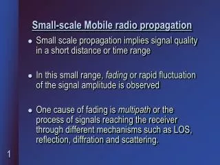
Small Scale Fading • Describes rapid fluctuations of the amplitude, phase of multipath delays of a radio signal over short period of time or travel distance • Caused by interference between two or more versions of the transmitted signal which arrive at the receiver at slightly different times. • These waves are called multipath waves and combine at the receiver antenna to give a resultant signal which can vary widely in amplitude and phase © İbrahim Körpeoğlu, 2002
Small Scale Multipath Propagation • Effects of multipath • Rapid changes in the signal strength • Over small travel distances, or • Over small time intervals • Random frequency modulation due to varying Doppler shifts on different multiples signals • Time dispersion (echoes) caused by multipath propagation delays • Multipath occurs because of • Reflections • Scattering © İbrahim Körpeoğlu, 2002
Multipath • At a receiver point • Radio waves generated from the same transmitted signal may come • from different directions • with different propagation delays • with (possibly) different amplitudes (random) • with (possibly) different phases (random) • with different angles of arrival (random). • These multipath components combine vectorially at the receiver antenna and cause the total signal • to fade • to distort © İbrahim Körpeoğlu, 2002
Multipath Components Radio Signals Arriving from different directions to receiver Component 1 Component 2 Component N Receiver may be stationary or mobile. © İbrahim Körpeoğlu, 2002
Mobility • Other Objects in the radio channels may be mobile or stationary • If other objects are stationary • Motion is only due to mobile • Fading is purely a spatial phenomenon (occurs only when the mobile receiver moves) • The spatial variations as the mobile moves will be perceived as temporal variations • Dt = Dd/v • Fading may cause disruptions in the communication © İbrahim Körpeoğlu, 2002
Factors Influencing Small Scale Fading • Multipath propagation • Presence of reflecting objects and scatterers cause multiple versions of the signal to arrive at the receiver • With different amplitudes and time delays • Causes the total signal at receiver to fade or distort • Speed of mobile • Cause Doppler shift at each multipath component • Causes random frequency modulation • Speed of surrounding objects • Causes time-varying Doppler shift on the multipath components © İbrahim Körpeoğlu, 2002
Factors Influencing Small Scale Fading • Transmission bandwidth of the channel • The transmitted radio signal bandwidth and bandwidth of the multipath channel affect the received signal properties: • If amplitude fluctuates of not • If the signal is distorted or not © İbrahim Körpeoğlu, 2002
Doppler Effect • Whe a transmitter or receiver is moving, the frequency of the received signal changes, i.e. İt is different than the frequency of transmissin. This is called Doppler Effect. • The change in frequency is called Doppler Shift. • It depends on • The relative velocity of the receiver with respect to transmitter • The frequenct (or wavelenth) of transmission • The direction of traveling with respect to the direction of the arriving signal. © İbrahim Körpeoğlu, 2002
Doppler Shift – Transmitter is moving The frequency of the signalthat is received behind the transmitter will be smaller The frequency of the signalthat is received in front of the transmitter will be bigger © İbrahim Körpeoğlu, 2002
Doppler Shift –Recever is moving S Dl X q Y d v A mobile receiver is traveling from point X to point Y © İbrahim Körpeoğlu, 2002
Doppler Shift • The Dopper shift is positive • If the mobile is moving toward the direction of arrival of the wave • The Doppler shift is negative • If the mobile is moving away from the direction of arrival of the wave. © İbrahim Körpeoğlu, 2002
Impulse Response Model of a Multipath Channel • The wireless channel charcteristics can be expressed by impulse response function • The channel is time varying channel when the receiver is moving. • Lets assume first that time variation due strictly to the receiver motion (t = d/v) • Since at any distance d = vt, the received power will ve combination of different incoming signals, the channel charactesitics or the impulse response funcion depends on the distance d between trandmitter and receiver © İbrahim Körpeoğlu, 2002
Basic Digital Signal Processing (DSP)Concepts Introduction to Signals and Systems
Signals and Systems • Discrete-Time Signals • Time-domain representation • Transform domain representation • Continuous Time Signals • Transformations • Fourier Transform • Laplace Transform • Z-transform • Systems • Linear Time Invariant (LTI) Systems • Time Varying Systems • Impulse Response of Systems © İbrahim Körpeoğlu, 2002
Discrete-Time Signals – Time Domain Representation Signals are represented as series of numbers called samples. A sample value is denoted with x[n]. (n is an integer). A discrete-time signal is represented by {x[n]}, which is also called a sequence. Example: {x[n]} = {…,-0.95, -0.2, 2.7, 1.1, -3.67, -0.7, 4.1, …} n=0 x[n] is called nth sample of the signal. X[n] could be a real number or complex number or an integer. If complex: {x[n]} = {Xre[n] + [Xim[n]} The signal may be finite length or infinite length. A sequence of samples can be extended by appending zeros. © İbrahim Körpeoğlu, 2002
Discrete-Time Signals – Time Domain Representation 3 2 … … 1 n -4 -3 - 2 -1 0 1 2 3 4 5 6 7 8 -1 -2 {x[n]} = {…, -2, 1, 3, 0, 2, 1, 0, -1, -2, -1, -2, 0, 2,…} © İbrahim Körpeoğlu, 2002
Operations on Sequences • A single-input, single output system operates on a sequence, called the • input sequence and develope an other sequence, called output sequence. • In some system, there may be more than one input and/or more than one • output. • Basic Operations Let x[n] and y[n] be two input sequences: • Modulation: w1[n] = x[n] · y[n] (product of the corresponding sample values) A device implementing modulation is called modulator. • Addition: w2[n] = x[n] + y[n] (sum of the corresponding sample values) A device implementing addition is called adder. • Multiplication: w3[n] = Ax[n] (multiply each sample by A). A device implementing multiplication is called multiplier. © İbrahim Körpeoğlu, 2002
Operations on Sequences • 4) Time-shifting: w4[n] = x[n-N], N is integer. • If N > 0, then this is a delaying operation • If N < 0, then this is a advancing operation • The device implementing delaying operation by one sample is called • unit delay, and a device implementing advancing operation by one sample is calledunit advance. • 5) Time-reversing (Folding): w6[n] = x[-n] • 6) Pick-off node provides multiple copies of same sequence. © İbrahim Körpeoğlu, 2002
Basic Operations on Sequences X + x[n] x[n] w1[n] w2[n] Adder Modulator y[n] y[n] w2[n] = x[n]+y[n] w1[n] = x[n]y[n] A z -1 x[n] x[n] w4[n] w3[n] Multiplier Unit Delay w4[n] = x[n-1] w3[n] = Ax[n] x[n] x[n]] z x[n] w5[n] Pick-off Node w5[n] = x[n+1] Unit Advance x[n] © İbrahim Körpeoğlu, 2002
Discrete-time System x[n-1] x[n-2] x[n-3] x[n] z-1 z-1 z-1 a1 a2 a3 a4 + y[n] y[n] = a1x[n] + a2x[n-1] + a3x[n-2] + a4x[n-3] © İbrahim Körpeoğlu, 2002
Periodic and Aperiodic Signal A sequence is periodic if: A sequence is aperiodic if it is not periodic. Periodic sequences will be denoted with ~ on top of them. © İbrahim Körpeoğlu, 2002
Energy and Power Signals © İbrahim Körpeoğlu, 2002
Basic Sequences • Unit Sample • Real Sinusoidal Sequences • Exponential Sequences • Complex Exponentials • Real and Imaginary parts • Real Exponentials © İbrahim Körpeoğlu, 2002
Unit Sample Sequence Also called as discrete-time impulse or the unit impulse. 1 0 0 The unit sample sequence shifted by k samples is given by: 1 0 k Any arbitrary sequence can be represented as the sum of weighted time-shifted unit sample sequences. Knowing the response of a LTI system to unit impulse, we can computeits response to any arbitrary input sequence. © İbrahim Körpeoğlu, 2002
Real Sinusoidal Sequence © İbrahim Körpeoğlu, 2002
Example – x[n] = 1.5cosw0n w0=0.1p w0=0.2p w0=0.9p w0=0.9p © İbrahim Körpeoğlu, 2002
Example – x[n] = 1.5cosw0n w0=1.1p w0=1.2p © İbrahim Körpeoğlu, 2002
Exponential Sequences © İbrahim Körpeoğlu, 2002
A complex exponential: real part © İbrahim Körpeoğlu, 2002
Real Exponentials X[n]=0.2(1.2)n a>1 Growing • X[n]=20(0.9)n • < 1 Decaying © İbrahim Körpeoğlu, 2002
Discrete-Time Systems • Given an input sequence, generates an output sequence. • If all signals are digital signals (which is the case for practical systems), then it is called a digital filter. • Classification • Linear System • Shift-Invariant System • Causal System • Stable System • Passive and Lossless Systems © İbrahim Körpeoğlu, 2002
Linear System A system where superposition principle always holds. © İbrahim Körpeoğlu, 2002
Shift-Invariant System If indices n is not related to specific time instants, then the system is called time invariant. This property ensures that for a specified input, the output of the system is independent of the time the input is applied. An LTI (Linear Time Invariant) System is a system that satisfies both linearity and time-invariance properties. © İbrahim Körpeoğlu, 2002
Other System Properties Causal System: In a causal discrete time system, the n0th output sample y[n0] depends only on input samples x[n] for n <= n0 and does not depend on input Samples for n > n0. Stable System: A discrete-time system is stable if and only if, for every bounded input, the output is also bounded. Passive and Lossless System: A disceret-time system is passive if, for every finite energy input sequence x[n], the output sequence y[n] has, at most, the same energy. A disceret-time system is lossless if, for every finite energy input sequence x[n], the output sequence y[n] has the same energy. © İbrahim Körpeoğlu, 2002
Impulse Response The response of a digital filter to a unit sample sequence {d[n]} is called the unit response, or simply, the impulse response, and denoted by: {h[n]} A linear time invariant system (filter) is completely characterized in the time-domain by its impulse response. Example: A system is given with the equation below: y[n] = a1x[n] + a2x[n-1] + a3x[n-2] + a4x[n-3] By setting x[n] = d[n], we can find out the impulse response of the system: h[n] = a1d[n] + a2d[n-1] + a3d[n-2] + a4d[n-3] {h[n]} = {a1, a2, a3, a4} © İbrahim Körpeoğlu, 2002
LTI: Input-Output Relationship {x[n]} = {…,0, 0, 0.5, 0, 0, 1.5, -1, 0, 1, 0, 0.75, 0, 0, …} An arbitrary sequence x[n]in the time domain can be represented as a weighted sum of some basic sequences and its delayed versions. A commonly used basic sequence is unit sample sequence (unit impulse). Sequence x[n] described above can be expressed as: © İbrahim Körpeoğlu, 2002
LTI: Input-Output Relationship LTI System d[n] Given h[n] (impulse response of the LTI system) LTI System Compute y[n] x[n] y[n] Lets compute the response of the this system (filter) to input x[n], where Since the system is time-invariant, the response to d[n-n0] will be h[n-n0]. Then: © İbrahim Körpeoğlu, 2002
LTI: Input-Output Relationship Any x[n] can be expressed as the weighted linear combination of delayed and advanced unit sample sequences as follows: x[k] denotes the kth sample value of {x[n]} By using the fact that the response of system to d[n-k] is h[n-k]. by change of variables is called convolution sum of x[n] and y[n] © İbrahim Körpeoğlu, 2002
Example © İbrahim Körpeoğlu, 2002
Unit Impulse and Response d(n) h(n) © İbrahim Körpeoğlu, 2002
Computation of Response x To compute y[n], multiple row labeled x[k] with row labeled h[n-k]. Example:To compute y[3] : multiply row numbered 1 with row numbered 6. = (-2x-1)+(0x0)+(1x2)+(-1x1)+(3x0) = 3 © İbrahim Körpeoğlu, 2002
Response © İbrahim Körpeoğlu, 2002
Response Sequence: y[n] x[n] y[n] {y[n]} = {…0,0,0,-2,-4,1,3,1,5,1,-3,0,0,0,…} The convolution of two finite-length sequences results in a finite-length sequence. © İbrahim Körpeoğlu, 2002
Simple Interconnection of Systems Cascade Connection: h1[n] h2[n] h2[n] h1[n] Parallel Connection h1[n] h1[n] © İbrahim Körpeoğlu, 2002
Classifications of LTI Discrete-Time Systems If h[n] is of finite length, such that h[n]=0 for n<N1 and n>N2, then the system is called finite impulse response (FIR) discrete time system. In this case, the convolution reduces to: If h[n] is of infinite length, then the system is called infinite impulse response (IIR) discrete-time system. For a causal system, the convolution is expressed as: © İbrahim Körpeoğlu, 2002
Random Signals • Deterministic Signal: They can be uniquely determined by a mathematical expression or a table lookup. • Random Signal (Stochastic Signal): Each sample value is generated in a random fashion. • A discrete time random signal consists of a typically infinite collection (or ensemble) of discrete time sequences {X[n]}. • At any given time index n, the observed sample value x[n] is the value taken by the random variable X[n]. • A random process is a family of random variables {X[n]}. © İbrahim Körpeoğlu, 2002
Power of Discrete-Time Random Signals © İbrahim Körpeoğlu, 2002
Continuous Time Signals Continues Time Impulse: The Unit Impulse d(t) is continues time signal that has the value ∞at time t=0, and zero for all other time t. de(t) approximates d(t). δe(t) 1/ε The area under the spike is 1 t 0 ε/2 -ε/2 © İbrahim Körpeoğlu, 2002