Download
1 / 42
420 likes | 580 Views
Viewing. Chapter 5. Introduction: We have completed our discussion of the first half of the synthetic camera model specifying objects in three dimensions We now investigate the multitude of ways in which we can describe our virtual camera.

E N D
Viewing Chapter 5
Introduction: • We have completed our discussion of the first half of the synthetic camera model • specifying objects in three dimensions • We now investigate the multitude of ways in which we can describe our virtual camera. • First, we look at the types of views we can create, and why we need more than one type of view. • Then we examine how an application viewer can create a particular view in within OpenGL. Chapter 5 -- Viewing
1. Classical Computer Viewing • Before looking at the interface between computer graphics systems and application programmers for 3D viewing, we take a slight diversion to consider classical viewing. • There are two reasons to do this • First, many jobs that were formerly done by hand drawing - such as animation in movies, architectural rendering, .. Are now done routinely with the aid of compute graphics. • Practitioners of these fields need to produce classical views. Chapter 5 -- Viewing
Second, the relationship between classical and computer viewing shows many advantages of, and a few difficulties with, the approach used by most APIs. • When we introduced the synthetic camera model in Chapter 1, we covered some elements: • objects, viewers, projectors, and a projection plane • Figure 5.1 • The projectors meet at the center of projection (COP) • this corresponds to the center of the lens in the camera, or in the eye Chapter 5 -- Viewing
Both classical and computer graphics allow the viewer to be an infinite distance from the objects • Note, as we move the COP to infinity, the projectors become parallel and the COP can be replaced with a direction of projection (DOP) • Figure 5.2 Chapter 5 -- Viewing
Although computer graphics systems have two fundamental types of viewing • (parallel and perspective), • classical graphics appears to permit a host of different views ranging from: • multiview orthographic projections, one- two- and three-point perspectives • This seeming discrepancy arises • in classical graphics due to the desire to show a specific relationship among an object, the viewer, and the projection plane • as opposed to the computer graphics approach of complete independence of all specifications Chapter 5 -- Viewing
1.1 Classical Viewing • When an architect draws an image of a building, • they know which sides they wish to display, • and thus where they should place the viewer • Each classical view is determined by a specific relationship between the objects and the viewer. • Figure 5.3 Chapter 5 -- Viewing
1.2 Orthographic Projections • The classical Orthographic projection • Figure 5.4 • Multiview Orthographic projections • Figure 5.5 Chapter 5 -- Viewing
1.3 Axonometric Projections • If we allow the projection plane to be at any angle (not just parallel with a face of the object) we end up with an axonometric view. • Figure 5.6 • Figure 5.7 Chapter 5 -- Viewing
1.4 Oblique Projections • These are the most general parallel views • projectors can make an arbitrary angle with the projection plane. • Figure 5.8 Chapter 5 -- Viewing
1.5 Perspective Viewing • All perspective views are characterized by diminution of size. • (the farther away, the smaller they are) • Figure 5.9 Chapter 5 -- Viewing
2. Positioning of the Camera • We can now return to 3D graphics from a computer perspective • We now examine the API that OpenGL provides for three-dimensional graphics, and show how other APIs differ • In this section we deal with positioning the camera. • In Section 5.4 we discuss how we specify the desired projection. Chapter 5 -- Viewing
In OpenGL, the model-view and projection matrices are concatenated together to form the matrix that applies to geometric entities such as vertices. • We have seen how to use the model-view matrix • to position objects in space. • The other is to convert from the reference frame used for modeling to the frame of the camera Chapter 5 -- Viewing
2.1 Positioning of the Camera Frame • Initially the camera is at the origin • Figure 5.11 • Consider this sequence • Figure 5.12 Chapter 5 -- Viewing
At any given time, the state of the model-view matrix encapsulates the relation between the camera frame and the world frame. • Although combining the modeling and viewing transformations into a single matrix may initially cause confusion, on closer examination this approach is a good one. • The obvious next problems are how we specify the desired position of the camera and how we implement camera positioning in OpenGL Chapter 5 -- Viewing
Here, we find it convenient to think in terms of moving the default camera relative tot he world frame. • We will outline three approaches to this. • The First Approach: • Specify the position indirectly by applying a sequence of rotations and translations to the model-view matrix • This is a direct application of the instance transformations we presented in Chapter 4 Chapter 5 -- Viewing
We must be careful for two reasons: • First, we usually want to define the camera before we position the objects in the scene. • Second, transformations on the camera may appear to be backward from what we might expect. • Figure 5.13 • glMatrixMode(GL_MODELVIEW); • glLoadIdentity( ); • glTranslatef(0.0, 0.0, -d); • glRotatef(-90.0, 0.0, 1.0, 0.0) Chapter 5 -- Viewing
2.2 Two Viewing APIs • We can take a different approach to positioning the camera -- an approach used by PHIGS, ... • We describe the camera’s position and orientation in the world frame • It’s desired location is centered at the view-reference point (VRP) • It’s orientation is specified with the view-plane normal (VPN) and the vie-up vector (VUP • Figure 5.15 Chapter 5 -- Viewing
2.3 The Look-At Function • The use if the VRP, VPN, and VUP is but one way to provide an API for specifying the position of a camera. • In many situations, as more direct method is appropriate. • FIGURE 5.17 • gluLookAt(eyex, eyey, eyez, atx, aty, atz, upx, upy, upz); Chapter 5 -- Viewing
2.4 Other Viewing APIs • In many applications, neither of the viewing interfaces that we have presented is appropriate. • Consider a flight simulator: • The pilot worries about roll, pitch, and yaw • Figure 5.18 Chapter 5 -- Viewing
Viewing in many applications is most naturally specified in polar coordinates -- rather than rectilinear coordinates. • Applications involving objects that rotate about other objects fit this category. • Figure 5.19 Chapter 5 -- Viewing
3. Simple Projections • With a real camera, once we position it, we still must select a lens. • In computer graphics we select the type of lens and the size of the film by selecting the type of projection and the viewing parameters. • Most APIs distinguish between parallel and perspective views by providing different functions for the two cases. • In OpenGL we can set the projection matrix with a glLoadMatrix function, or we can other functions for the most common viewing conditions Chapter 5 -- Viewing
3.1 Perspective Projections • Suppose that we are in the camera frame with the camera located at the origin pointed in the negative z direction. • Figure 5.20 Chapter 5 -- Viewing
As we saw in Chapter 2, we can place the projection plane in front of the center of projection. If we do so, we get the following views: • Figure 5.21 Chapter 5 -- Viewing
3.2 Orthogonal Projections • Orthogonal or orthographic projections are a special case of parallel projections, in which the projectors are perpendicular to the view of the plane. • Figure 5.23 Chapter 5 -- Viewing
4. Projections in OpenGL • The projections we just developed did not take into account the properties of the camera: • the focal length of its lens, • the size of the film plane • View Volume • Figure 5.24 Chapter 5 -- Viewing
Most graphics APIs define clipping parameters through the specification of a projection. • The resulting view volume is a frustum --a truncated pyramid. • Figure 5.25 Chapter 5 -- Viewing
4.1 Perspectives in OpenGL • In OpenGL we have two functions for specifying perspective views and one for specifying parallel views. • We can specify our camera view by: • glFrustrum(xmin, xmax, ymin, ymax, near, far) • Figure 5.26 Chapter 5 -- Viewing
Because the projection matrix determined by these specifications multiplies the present matrix, we must first select the matrix mode. • A typical sequence is • glMatrixMode(GL_PROJECTION); • glLoadIdentity( ); • glFrustrum(xmin, xmax, ymin, ymax, near, far); Chapter 5 -- Viewing
In many applications, it is natural to specify the angle or field of view • gluPerspective(fovy, aspect, near, far); • Figure 5.27 Chapter 5 -- Viewing
4.2 Parallel Viewing in OpenGL • The only paralel-viewing function provided by OpenGL is the orthographic viewing function • glOrtho(xmin, xmax, ymin, ymax, near, far) • Figure 5.28 Chapter 5 -- Viewing
5. Hidden-Surface Removal • Hidden surface removal algorithms can be divided into two broad classes: • Object-space algorithms • attempt to order the surfaces of the objects in the scene such that drawing surfaces in a particular order provides the correct image. • Image-space algorithms • work as part of the projection process and seek to determine the relationship among object points on each projector • z-buffer fits into this category. Chapter 5 -- Viewing
The major advantage of z-buffer is • that its worst case complexity is proportional to the number of polygons. • It can be implemented with a small number of additional calculations over what we have to do anyway. • Figure 5.29 • Typically you use these functions: • glutInitDisplayMode(GLUT_DOUBLE | GLUT_RGB | GLUT_DEPTH); • glEnable(GL_DEPTH_TEST); • glClear(GL_DEPTH_BUFFER_BIT); Chapter 5 -- Viewing
6. Walking Through a Scene • Let us modify the version of our color-cube program from Chapter 4 • Old Version: • the cube rotated about the origin. • Orthographic projection • In this version • perspective projection • allow the camera to move. Chapter 5 -- Viewing
void keys(unsigned char key, int x, int y) • { • if(key == ‘x’) viewer[0] -= 1.0; • if(key == ‘X’) viewer[0] += 1.0; • if(key == ‘y’) viewer[1] -= 1.0; • if(key == ‘Y’) viewer[1] += 1.0; • if(key == ‘z’) viewer[2] -= 1.0; • if(key == ‘Z’) viewer[2] += 1.0; • } Chapter 5 -- Viewing
void display(void) • { • glClear(GL_COLOR_BUFFER_BIT | GL_DEPTH_BUFFER_BIT); • glLoadIdentity( ); • gluLookAt(viewer[0], viewer[1], viewer[2], • 0.0, 0.0, 0.0, 0.0, 1.0 , 0.0); • glRotatef(theta[0], 1.0, 0.0, 0.0); • glRotatef(theta[1], 0.0, 1.0, 0.0); • glRotatef(theta[2], 0.0, 0.0, 1.0); • colorcube( ); • glFlush( ); • glutSwapBuffers( ); • } Chapter 5 -- Viewing
void myReshape(int w, int h) • { • glViewport(0,0,w,h); • glLoadMatrix(GL_PROJECTION); • glLoadIdentity( ); • if(w<=h) • glFrustrum(-2.0, 2.0, -2.0 * (Glfloat)h/(Glfloat)w, • 2.0*(Glfloat(h)/(Glfloat)w, 2.0, 20.0); • else • glFrustrum(-2.0, 2.0, -2.0 * (Glfloat)w/(Glfloat)h, • 2.0*(Glfloat)w/(Glfloat)h, 2.0, 20.0); • glMatrixMode(GL_MODELVIEW); • } Chapter 5 -- Viewing
9. Projections and Shadows • The creation of simple shadows is an interesting application of projection matrices. • This section covers how to re-project the polygon casting the shadow onto the ground • this re-projection is called a shadow polygon. Chapter 5 -- Viewing
For a simple environment, this technique works well, however, when objects cast shadows on other objects, this method becomes impractical. • In chapter 9 we address a more general shadow-creation method that requires more work. Chapter 5 -- Viewing
10. Summary • We have come a long way. • We can now write complete, nontrivial, three dimensional applications. • Probably the most instructive activity that you can do now is to write such an application. • In Chapter 6 we consider the interaction of light with the materials that characterize our objects. Chapter 5 -- Viewing
11. Suggested Readings • Foley (90), Watt (93) and Hern&Baker (94) derive canonical projection transformations • All follow the PHIGS orientation, so the API is slightly different from the one used here. • Most differ in whether they use column or row matrices, in where the COP is located, and in whether the projection is in the positive or negative z direction. • See the OpenGL Programmer’s Guide (97) for further discussion of the use of the model-view and projection matrices Chapter 5 -- Viewing
Exercises -- Due next class Chapter 5 -- Viewing