Download
1 / 33
340 likes | 496 Views
CHE 536 ENGINEERING OPTIMIZATION . COURSE POLICIES AND OUTLINE Prof. Shi-Shang Jang Chemical Engineering Department National Tsing-Hua University Hsinchu Feb. 2011. Instructor: Prof. Shi-Shang Jang . Class Meeting: Every Thursday, 2:00-5:00

E N D
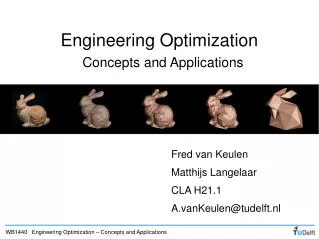
CHE 536 ENGINEERING OPTIMIZATION COURSE POLICIES AND OUTLINE Prof. Shi-Shang Jang Chemical Engineering Department National Tsing-Hua University Hsinchu Feb. 2011
Instructor: Prof. Shi-Shang Jang • Class Meeting: Every Thursday, 2:00-5:00 • Classroom: Rm#221, Chem. Engng. Buldg. • Textbook : P. Venkataraman, Applied Optimization with MATLAB Programming. Wiley-Interscience, 2001 • References: • Reklaitis, Ravindran and Ragsdell, Engineering Optimization, Methods and Applications, .Wiley, 1983. • Vanderplaats, G.N., Numerical Optimization Techniques for Engineering Design with Applications, McGraw-Hill International , 1993. • Optimization of Chemical Processes, 2nd Ed., Edgar, Himmelblau and Lasdon, McGraw-Hill, Boston, 2001 • Course Objective: • To learn problem formulation of optimization. • To realize the algorithms of numerical methods of optimization. • To know the applications of numerical optimization.
Policies • Homework Policy: Biweekly (computer programming) homework, due at next week class meeting. No late homework will be accepted. • Grading Policy:Homework :30%, Midterm Exam: 35%, Term project: 35% • Lecture Notes: http://pie.che.nthu.edu.tw/
Course Outline • Course Orientation 2/24 • Introduction and Single Variable Optimization 3/3, 3/10 • Unconstrained Optimization 3/17, 3/24 • Linear Programming 3/31, 4/7 • Theoretical Concepts of Nonlinear Programming 4/14, 4/21 • Midterm Exam 4/28 • Generalized Reduced Gradient Approach 5/5,12,19 • Successive Quadratic Programming 5/26, 6/2 • Final Project Presentation 6/9
Chapter 1. INTRODUCTION Why optimized? Improve the process to realize maximum system potential; Attain improved designs; maximize profits; reduce cost of productions.
Essential features of optimization problem • An objective function is defined which needs to be either maximized or minimized. The objective function may be technical or economic. Examples of economic objective are profits, costs of production etc.. Technical objective may be the yield from the reactor that needs to be maximized, minimum size of an equipment etc.. Technical objectives are ultimately related to economics. • Underdetermined system: If all the design variables are fixed. There is no optimization. Thus one or more variables is relaxed and the system becomes an underdetermined system which has at least in principle infinite number of solutions.
Essential features of optimization problem- Continued • Competing influences: In most of the optimization problems, there would be some set of variables which has opposite influence on the objective function. Such competing influences require some balancing and hence result in typical optimization problems. • Restrictions: Usually the optimization is done keeping certain restrictions or constraints. Thus, the amount of row material may be fixed or there may be other design restrictions. Hence in most problems the absolute minimum or maximum is not needed but a restricted optimum i.e. the best possible in the given condition
Problem Statements Given a design vector An objective function f(x) A set of equality constraints g(x)=0 A set of inequality constraints, h(x)0 The general problem formulation:
Examples- An Inspector Problem (Linear Programming): • Assume that it is desired to hire some inspectors for monitoring a production line. A total amount of 1800 species of products are manufactured every day (8 working hours), while two grades of inspectors can be found. Maximum, 8 grade A inspector and 10 grade B inspector are available from the job market. Grade A inspectors can check 25 species/hour, with an accuracy of 98 percent. Grade B inspectors can check 15 species/hour, with an accuracy of 95 percent. The wage of a grade A inspector is $4.00/hour, and the wage of a grade B inspector is $3.00/hour. What is the optimum policy for hiring the inspectors?
Problem Formulation • Assume that the x1grade A inspectors x2 grade B inspects are hired, then • total cost to be minimized • 48x1+38 x2+2580.022x1+1580.052x2 =40 x1+36 x2 • manufacturing constraint • 258x1+158x21,800 200 x1+120 x21,800 • no. of inspectors available: • 0 x18 • 0 x210
Example – optimal pipe diameter • In a chemical plant, the cost of pipes, their fittings, and pumping are important investment cost. Consider a design of a pipeline L feet long that should carry fluid at the rate of Q gpm. The selection of economic pipe diameter D(in.) is based on minimizing the annual cost of pipe, pump, and pumping. Suppose the annual cost of a pipeline with a standard carbon steel pipe and a motor-driven centrifugal pump can be expressed as: Formulate the appropriate single-variable optimization problem for designing a pipe of length 1000ft with a fluid rate of 20gpm. The diameter of the pipe should be between 0.25 to 6 in.
The MATLAB Code for Process Design Example • d=linspace(0.25,6); • l=1000;q=20; • for i=1:100 • hp=4.4e-8*(l*q^3)/d(i)^5 + 1.92e-9*(l*q^2.68) /(d(i)^4.68); • f(i)=0.45*l+0.245*l*d(i)^1.5+3.25*hp^0.5+61.6*hp^0.925+102; • end cost diameter
Examples- A Chemical Reactor Design Problem Material Balances: Energy Balances:
Examples- A Chemical Reactor Design Problem - Continued • Problem: Assume that C0, TJ, tf can be designed, it is our objective to find good settings such that CB(tf) can be maximized
Special Types of NLP problems • Unconstrained optimization • In here, neither equality nor inequality constraint exists • Linear Programming (LP) • In here, all the objective function and constraints are linear functions to x.
Special Types of NLP problems - Continued • Quadratic Programming (QP) In here, only the objective function is quadratic, but the constraints are linear
Special Types of NLP problems - Continued • Optimization with respect to a continuous variable (Calculus of Variation) Find x(t) such that is minimized
Special Types of NLP problems - Continued • Dynamic Programming (DP) Here, xi represents the state of the system in the ith stage and ui is some decision variable, i.e. some decision taken at the ith stage. The values of xi and ui determine uniquely xi+1: Here, it is assumed that x0 is known, when the state of the system changes from xi to xi+1, there is an improvement or degradation in an objective function as cost or profit. Let this be J=f(xi,ui,i) , then the cumulative profit over N stages is:
Special Types of NLP problems - Continued • Integer Programming (IP): • Some of the variables are constrained to take integer values. As x0 is fixed the magnitude of the cumulative profit is determined only by the various decisions taken ui (i=0 to N-1). Hence Jc is to be optimized with respect to ui. Now, constraints may be imposed on xi and ui. This constitutes a dynamic programming (DP)
The Iterative Optimization Procedure – A Basic Idea • Optimization is basically performed in a fashion of iterative optimization. We give an initial point x0, and a direction s, and then perform the following line search: where * is the optimal point for the objective function and satisfies all the constraints. Then we start from x1 and find the other direction s’, and perform a new line search until the optimum is reached.
Terminology • Contour plot
Terminology - Continued • Global optimum v.s. Local optimum
Terminology - Continued • Convex v.s. Concave functions • A function (x) is called convex over the domain R if for all x1, x2R, and 0<<1, then • If the inequality holds, the function is called strictly convex. A concave function is a function that cannot have a value smaller than that obtained by a linear approximation.
Terminology - Continued • Unimodal function • If the function increases up to a maximum then decreases for all other values, it is called a unimodal function • Gradient and Hessian of a function • Gradient of a function f(x) is defined by a column vector of the first partial derivatives of f(x) with respect to each variables x1 to xn evaluated at some x • Hessian matrix of f(x) is defined as the symmetric square matrix of second partial derivatives
Terminology - Continued • Feasible Regions- • Region of search. • The region bounded by the inequality and equality constraints. • Convex region of search (not convex function): • A convex region is one region such that a line joining any two points lying in the region.
Appendix – Mesh and Contour • 3-dimensional plot and contour plot are important to demonstrate the optimality of a function • Internal functions of MATLAB: mesh(x,y,z) and meshgrid are useful in this case
Function MeshGrid • To Produce two arrays containing duplicates of its inputs so that all combinations of its inputs are considered. xtest=1:5; ytest=6:9; [xx,yy]=meshgrid(xtest,ytest) xx = 1 2 3 4 5 1 2 3 4 5 1 2 3 4 5 1 2 3 4 5 yy = 6 6 6 6 6 7 7 7 7 7 8 8 8 8 8 9 9 9 9 9
Mesh plot of function z=x^2+y^2 • for i=1:100 • for j=1:100 • z(i,j)=xx(i,j)^2+yy(i,j)^2; • end • end • mesh(xx,yy,z)
Contour plot of function z=x^2+y^2 • contour(xx,yy,z)
Himmelblau’s Function • function y=himmel(x1,x2) • y=(x1*x1+x2-11)^2+(x1+x2*x2-7)^2; • x1=linspace(-5,5,21); • x2=linspace(-5,5,21); • for i=1:21 • for j=1:21 • zz(i,j)=himmel(x1(i),x2(j)); • end • end; • mesh(x1,x2,zz);