Download
1 / 37
430 likes | 661 Views
Concepts and Applications. Engineering Optimization. Fred van Keulen Matthijs Langelaar CLA H21.1 A.vanKeulen@tudelft.nl. Contents. Optimization problem checking and simplification Model simplification. Expensive model. Cheap model. Optimizer. Optimizer. Model simplification.

E N D
Concepts and Applications Engineering Optimization Fred van Keulen Matthijs Langelaar CLA H21.1 A.vanKeulen@tudelft.nl
Contents • Optimization problem checking and simplification • Model simplification
Expensivemodel Cheapmodel Optimizer Optimizer Model simplification • Basic idea: • Motivation: • Replacement of expensive function, evaluated many times • Interaction between different disciplines • Estimation of derivatives • Noise
Procedure: Extract information Construct approximation Model simplification (2) • Drawback: loss of accuracy • Different ranges: local, mid-range, global • Synonyms: • Approximation models • Metamodels • Surrogate models • Compact models • Reduced order models
Model simplification (3) • Information extraction: linked to techniques from physical experiments: “plan of experiments” / DoE • Many approaches! Covered here: • Taylor series expansions • Exact fitting • Least squares fitting (response surface techniques) • Kriging • Reduced basis methods • Briefly: neural nets, genetic programming, simplified physical models • Crucial: purpose,range and level of detail
Taylor series expansions • Approximation based on local information: Truncation error! Use of derivative information! Valid in neighbourhood of x
20th order 4th order 3rd order 5th order 2nd order Taylor approximation example Function Approximation(x = 20) 1st order x
Exact fitting (interpolation) • # datapoints = # fitting parameters • Every datapoint reproduced exactly • Example: f2 f1 x1 x2
Often used: polynomials, generalized polynomials: Exact fitting (2) • Easy for intrinsically linear functions: No smoothing / filtering / noise reduction Danger of oscillations with high-order polynomials
9th order polynomial 5th order 9th order Oscillations • Referred to as “Runge phenomenon” In practice: use order 6 or less
“Best fit”? Minimize sum of squared deviations: Least squares fitting • Less fitting parameters than datapoints • Smoothing / filtering behaviour • “Best fit”? Minimize sum of deviations: f x
Short notation: Least squares fitting (2) • Choose fitting function linear in parameters ai :
LS fitting (3) • Minimize sum of squared errors:(Optimization problem!)
Polynomial LS fitting • Polynomial of degree m:
quadratic 6th degree Polynomial LS example 1.2 samples 1 0.8 0.6 0.4 0.2 0 -0.2 -1 -0.8 -0.6 -0.4 -0.2 0 0.2 0.4 0.6 0.8 1
Multidimensional LS fitting • Polynomial in multiple dimensions: Number of coefficients ai for quadratic polynomial in Rn: Curse of dimensionality!
x3 x2 x1 Fractional factorial design 2n full factorial design Response surface • Generate datapoints through sampling: • Generate design points through Design of Experiments • Evaluate responses Fit analytical model Check accuracy
Latin Hypercube Sampling (LHS) • Popular method: LHS • Based on idea of Latin square: • Properties: • Space-filling • Any number of design points • Intended for box-like domains • Matlab: lhsdesign
Statistical quality indicators: • R2 correlation measure: • F-ratio (signal to noise): Okay: >0.6 Okay: >>1 (LS) Fit quality indicators • Accuracy? More / fewer terms? • Examine the residuals • Small • Random! e 0 xi
Nonlinear LS: more complicated functions of ai: More difficult to fit! (Nonlinear optimization problem) Matlab: lsqnonlin Nonlinear LS • Linear LS: intrinsically linear functions (linear in ai):
LS pitfalls f • Scattered data: • Wrong choice of basis functions: x f x
Kriging • Named after D.C. Krige, mining engineer, 1951 • Statistical approach: correlation between neighbouring points • Interpolation by weighted sum: • Weights depend on distance • Certain spatial correlationfunction is assumed(usually Gaussian)
Kriging properties • Kriging interpolation is “most likely” in some sense (based on assumptions of the method) • Interpolation: no smoothing / filtering • Many variations exist! • Advantage: no need to assume form of interpolation function • Fitting process more elaborate than LS procedure
Kriging example • Results depend strongly on statistical assumptions and method used: Kriging interpolation Dataset z(x,y)
Select small number of “modes” to build basis • Example: eigenmodes Reduced order model • Idea: describing system in reduced basis: • Example: structural dynamics
N1 Nk k1 • Reduced system equations: kN NN Nk kN N1 Reduced order model (2) • Reduced basis:
Reduced order models • Many approaches! • Selection of type and number of basis vectors • Dealing with nonlinearity / multiple disciplines • Active research topic • No interpolation / fitting, but approximate modeling
Structural model Mass model Aerodynamic model Example:Aircraft model
f(x) output S(input) Neural nets x To determine internal neuron parameters, neural nets must be trained on data.
Neural net features • Versatile, can capture complex behavior • Filtering, smoothing • Many variations possible • Network • Number of neurons, layers • Transfer functions • Many training steps might be required (nonlinear optimization) • Matlab: see e.g. nndtoc
^2 + / x3 x1 x2 Genetic programming • Building mathematical functions using evolution-like approach • Approach good fit by crossover and mutation of expressions
Genetic programming • LS fitting with population of analytic expressions • Selection / evolution rules • Features: • Can capture very complex behavior • Danger of artifacts / overfitting • Quite expensive procedure
Refinement: correction function, parameter functions ... Simplified model Correctionfunction f(x) x Simplified physical models • Goal: capture trends from underlying physics through simpler model: • Lumped / Analytic / Coarse • Parameters fitted to “high-fidelity” data
Model simplification summary Many different approaches: • Local: Taylor series (needs derivatives) • Interpolation (exact fit): • (Polynomial) fitting • Kriging • Fitting: LS • Approximate modeling: reduced order / simplified models • Other: genetic programming, neural nets, etc
Expensivemodel Cheapmodel Optimizer Optimizer Response surfaces in optimization • Popular approach for computationally expen-sive problems: • DoE, generate samples (expensive) in part of domain • Build response surface (cheap) • Perform optimization on response surface (cheap) • Update domain of interest, and repeat Additional advantage: smoothens noisy responses Easy to combine with parallel computing
Optimum (Expensive) simulation Sub-optimal point Trust region Response surface Example: Multi-point Approximation Method Design domain