Download
1 / 35
350 likes | 489 Views
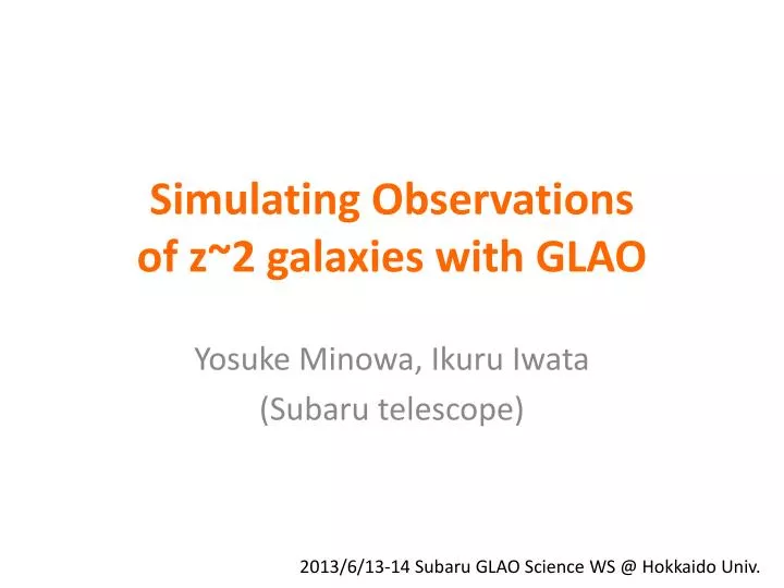
Simulating Observations of z~2 galaxies with GLAO. Yosuke Minowa, Ikuru Iwata (Subaru telescope). 2013/6/13-14 Subaru GLAO Science WS @ Hokkaido Univ. Motivation. What is the most unique capability of the GLAO instrument?

E N D
Simulating Observations of z~2 galaxies with GLAO Yosuke Minowa, Ikuru Iwata (Subaru telescope) 2013/6/13-14 Subaru GLAO Science WS @ Hokkaido Univ.
Motivation • What is the most unique capability of the GLAO instrument? • GLAO will start observation from somewhere around 2020 • It is important to think about the uniqueness of the Subaru GLAO comparing to TMT and any other space based telescope. • Evaluate the competitiveness of GLAO imager, MOS spec., and IFU spec. • Case study for z~2 galaxies by simulating the actual observations.
Science requirement: Sensitivity SINFONI spectroscopic survey of z~2 star forming galaxies (Forster Schreiber+09) • Can we detect Hα emission line corresponds to SFR ~ 1-10 Msun/yr to study < 10 10Msun galaxies? (Newman+13)
Science requirement: Spatial Resolution Star-forming galaxies (Forster-Schreiber+11) Seeing (0”.5) GLAO (0”.2) AO188 (0”.1) Bowens+04 (Size evolution of UV-dropout galaxies) TMT (0”.01) Redshift • Can we spatially resolve ~1kpc scale star-forming clumps at z~2? • Can we reconstruct morphological parameters of z~2 galaxies?
Simulating GLAO observation of z~2 galaxies • z~2 galaxy sample selection • HST/WFC3 H-band (F160W) image of z~2 galaxies • Highest resolution image currently available • Data from CANDELS (Koekemoer et al. 2011) GOODS-S surveywhose survey area (~120arcmin2) is comparable to the GLAO instrument • Selected KAB<23.9 BzK galaxies from MUSYC(Cardamone et al. 2010) catalog • z=2.1-2.6 star-forming BzK with spec-z: 40 --- K-band imaging/spectroscopy • z=1.3-1.7 passive-BzK with phot-z: 6 --- H,K-band imaging/spectroscopy
GLAO galaxy simulation recipe • Extracted galaxy morphological parameters --- Sersic profile fit: Effective radius Re, Sersic index N, Axis ratio, and Position angle ※ Simple convolution of the WFC3 image may not reproduce well the GLAO image since WFC3 spatial resolution (FWHM~0”.18) is worse than the best GLAO resolution (FWHM~0”.15). • Construct the model galaxy image from the morphological parameters without any PSF convolution. • Convolve the model galaxy image with the GLAO PSF • Add noise corresponds to 5 hrs integration We used 5hrs integration time and 5sigma S/N for all simulation, so as to evaluate the limitation in just 1 night observation.
Star-forming BzK at z=2.1-2.6 (Model) Comparison with z~2 sBzK sample at GOODS-N (Yuma et al. 2011) Modeling sBzK galaxies based on GOODS-S WFC3 image (CANDELS) Our sample Effective radiuslog(Re[kpc]) z=0 WFC3 Model Residual Stellar mass log(M*/Msun) Sersic profile
GLAO PSF (from Oya-san’s talk) We used the center PSF at the moderate seeing condition to simulate the observation of z~2 galaxies. Seeing condition: Bad (75%) : 0”.56@K Moderate (50%): 0.44@K Good (25%): 0”.35@K
PSF for each target field • Subaru Deep Field (Dec =+27.5deg) Apr, z=15deg • COSMOS (Dec=+2.2deg) Feb, z=15deg • SXDF/UDS (Dec=-5.2deg) Oct, z=30deg (from Oya-san)
Simulated Observations • Wide Field NIR imaging • Broad-band (BB) imaging • Narrow-band (NB) imaging • Multi-Object Slit (MOS) spectroscopy • Emission line • Continuum • Multi-IFU spectroscopy • Emission line
Imager Baseline Specification • Wider than any NIR imager on 8m class telescopes • The instrument throughput is assumed to be same as VLT/HAWK-I (~60%@JH, ~50%@K) • Seeing performance is just same as VLT/HAWK-I
Broad-band imaging: Sensitivity Passively evolving galaxies at z~1.5 (H-band) Star-forming galaxies at z~2 (Ks-band)
BB imaging: Possibility for reconstructing the morphological parameters with GLAO imager
BB imaging: summary • Simulated z~2 galaxy imaging in H, K-band with new GLAO PSF which takes into account the PSF difference according to the zenith angle and seasonal seeing change. • The point source sensitivity gain against the normal seeing instruments (such as VLT/Hawk-I) is different for each field. (1.0 mag for SDF, 0.7 mag for COSMOS) • The sensitivity gain for galaxies are almost same for all fields. • 0.3-0.6 mag for compact galaxies (<3kpc). • Hereafter, we used COSMOS PSF to simulate the observations of z~2 galaxies. • The limiting mag. is more than 3 magnitude brighter than TMT or JWST (~30mag in K, Wright et al. 2010). • Broad band imaging cannot be competitive • Wide-field capability might be useful for finding rare objects like passively evolving galaxies. • Morphological parameters (Re, N) can be reconstructed from the GLAO image for galaxies whose mass is larger than 1010Msun • For lower mass galaxies 109Msun, we can reconstruct size (Re), but cannot reconstruct Sersic index.
Narrow-band imaging: Hα map • Simulated Brγ-image of Hα emitters at z=2.3 with 5hrs integration • made from HST/WFC3 images of star-forming galaxies in SXDF (Tadaki+13) log(M*/Msun) ~ 8.9 SFR ~ 90 Msun/yr log(M*/Msun) ~ 10.8 SFR ~ 300 Msun/yr log(M*/Msun) ~ 11.2 SFR ~ 230 Msun/yr GLAO ~ 3”.0 Seeing S/N: 1 2 3 4 5 6 7 8 9 10
NB imaging: Summary • Star-forming clumps in galaxies can be clearly resolved with GLAO NB imaging. • GLAO can reach about 0.3-0.6 mag deeper than VLT/HAWK-I for compact galaxies (<3kpc) • Brγ-imaging can reach Hα emitters with SFR < 10Msun/yr for compact galaxies with re < 3kpc. • Wide field NB-imaging can be a good sample provider for the IFU study with TMT • JWST/NIRCAM (F212N) can reach about 1.8 mag deeper than GLAO NB image for galaxies with re~2kpc and more for point sources (from Iwata-san’s calculation). • More than 100hrs integration required to achieve similar depth as JWST/NIRCAM. • Legacy type survey could achieve this integration.
Multi-Object Slit Spectrograph Baseline Specification • Keck/MOSFIRE type instrument with 13’x13’ FOV • Wider FOV than any existing MOS spectrograph on 8m class telescopes • Assume similar throughput as Keck/MOSFIRE • the highest throughput ever achieved (30-40%@JHK) • Seeing performance is just same as Keck/MOSFIRE • Slit width is assumed to be 0”.4 which is 2 times wider than GLAO PSF.
MOS Spec.: emission line sensitivity • Emission line 5σ sensitivity for point source and extended source (Re~1kpc or ~ 0”.12 and N=1) with 5hrs integration.
MOS Spec.: Emission line sensitivity (Point Source) (Extended Source) • S/N of Hα emission line flux which corresponds to SFR~ 1 Msun/yr (assume E(B-V)=0.2) with 5hrs integration
MOS spec.: Continuum Sensitivity • Continuum 5 σ sensitivity for point and extended source with 5hrs integration
MOS. Spec: Summary • Emission line: GLAO can increase the S/N of emission lines by 2 times higher than MOSFIRE. • SFR~1Msun/yr can be detected with Ha emission line located between sky emission line. • Provides better sensitivity than NB-imaging, which enables redshift confirmation of the Ha-emitter discovered by NB imaging. • Although TMT can achieve 3 times better S/N than GLAO (based on Law et al. 2006), the MOS capability is still required to enable rapid follow-up of the target discovered by GLAO NB imaging. • Continuum sensitivity is worse than K~23mag. Follow-up spectroscopy of z~2 passive galaxies discovered by BB imaging should be done by TMT.
Multi Object IFU Baseline Specification • VLT/KMOS type multi-IFU • Throughput is assumed to be 80% of MOSFIRE due to the optical components for IFUs.
Multi-IFU: mock image • Simulated IFU S/N map of Hα emitters at z~2.3 • same objects as we used for NB imaging 1”.75x1”.75 GLAO Seeing
Multi-IFU: Sensitivity Re=1.4kpc S/N Re=3.0kpc SFR=1Msun/yr can be detected with S/N=5 for galaxies Re=1.4kpc Star Formation Rate [Msun/yr]
Multi-IFU: Summary • Star-forming cramps can be resolve with IFU. • GLAO IFU spectrograph can be detected Hα emission line from z~2 galaxies corresponds to SFR~ 1Msun/yr, if size of galaxies is less than 2 kpc. • TMT/IRIS can detect SFR~1Msun/yr from similar size galaxies with S/N>40 (Wright et al. 2010) • To be competitive with TMT/IRIS, GLAO IFU should have multiplicity of targets with more than 64 pick-off arm. • Need to investigate if this number is technically possible.
Conclusion Competitive less competitive Competitive??? (in Japanese 微妙) • Broad band imaging is not very competitive against the TMT/JWST, although >0.5mag gain can be obtained from the normal seeing instrument. • NB imaging can reach the galaxies with SFR <10 Msun/yr, which can be good targets to follow-up with TMT IFU. • Emission line sensitivity is only 3 times worse than TMT/IRIS, which could be competitive by combining with the GLAO NB imaging survey. • Continuum sensitivity is less competitive as we can detect galaxies brighter than 23 mag in K-band. • Multiple-IFU could be competitive against TMT/IRIS if we can have more than 60 pick-off arms , but it is better to invest TMT/IRMOS. Any comment or request for the simulations of GLAO observations are welcome.
Star-forming BzKs at z=2.1-2.6 (GLAO image) • Assuming 5 hours integration in K-band under moderate seeing condition (0”.5) GLAO Seeing (0”.5) 1.5@r=0”.2 1.5@r=0”.2 1.5@r=0”.2 2.5@r=0”.2 1.5@r=0”.2 1.5@r=0”.2 2.02 1.29 1.27 1.28 1.29 1.29 MUSYC 34852: zspec=2.32, H=22.5, K=21.9, log (M*/Msun)=11.1, Re=1.4[kpc], N=1.7
Passive BzKs at z=1.3-1.7 (Model) Comparison with the other z~2passive galaxies at HUDF (Cassata et al. 2010) Modeling pBzK galaxies from GOODS-S WFC3 image (CANDELS) Our sample Effective radius Re(Kpc) z=0 WFC3 Residual Model Stellar mass (M*/Msun)
Passive BzKs at z=1.3-1.7 (GLAO image) • Assuming 5 hours integration in H band under moderate seeing condition (0”.5) GLAO Seeing (0”.5) 1.6@r=0”.2 1.6@r=0”.2 1.6@r=0”.2 2.8@r=0”.2 1.6@r=0”.2 1.4@r=0”.2 2.49 1.26 1.33 1.30 1.31 1.30 MUSYC 37269: zphot=1.74, H=22.4, K=21.7, log (M*/Msun)=11.1, Re=1.1[kpc], N=1.7
BB imaging: Morphological study Sersic index (n) Log(re) [kpc] (Wuyts+2011)