FFT Accelerator Project

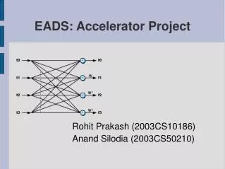
FFT Accelerator Project 4th October, 2007 Rohit Prakash (2003CS10186) Anand Silodia (2003CS50210)

FPGA: Overview • Work done • Structure of a sample program • Ongoing Work • Next Step

FPGA : work done • Register handling and console IO • Modified simple.c • Implemented an adder • Used VirtualBase member of ADMXRC2_SPACE_INFO • Registers can be indexed using (23 downto 2) bits of LAD (local address/data) signal when it is used to address the fpga

Structure of simple.vhd entity simple is port( All the local bus signals required); end simple architecture …

Ongoing work : ZBT • Structure of zbt_main seems to be similar to simple.c • zbt.vhd is a wrapper for zbt_main.vhd • Same port names defined in the same way and port mapped to each other • Do not understand the reason for this wrapper • C code not available in ADMXRC2 demos • Lalit’s code also uses zbt and block rams, so looking at his C and vhdl code

Next Step • To work with zbt and block RAMs • FFT implementation on the FPGA

Multiprocessor FFT Overview • Some improvements to the existing code • Improve the theoretical model • Compare theoretical run-time with actual run time • Statistics of each processor • Further refinement: Using BSP model • Pointers for Cache Analysis

Optimizations to the code • Removed other arrays (reducing memory references considerably) • Twiddle factors • Bit reversal addresses • Bit reversal faster using bit operations O(1) for each address calculation • All multiplications/divisions involving 2 implemented using shift operations O(1) • Power (2^n) in constant time using bit operations O(1)

Previously…

Now…

Improvement • For larger input size, our program (radix-2) is comparable to FFTW • Our program might surpass FFTW • Using SIMD • Higher radix (e.g. 4,8,16) • Coding in C

Redefining the execution time • For p processors, the total execution time is : (TN/p) + (1 – 1/p)(2N/B + KN) • p is a power of 2 • This assumes “RAM Model” • Assumes a flat memory address space with unit-cost access to any memory location • We did not take into account the memory hierarchy • E.g. matrix multiplication actually takes O(n5) instead of expected O(n3) [Alpern et al. 1994]

Redefining the execution time • Some observations • If the #processors are p , then the actual FFT computed if FFT(N/p)  time taken is TN/pand NOT TN/p • Time taken to combine (O(n) in RAM model) should be taken as: ΣKN/2i (i = 1 to log p) • NOT included the synchronization time • Currently looking execution time only from the perspective of master processor • The overheads for establishing sends and receives have been neglected (on measuring this (using ping-pong approach) the time was negligible

New Theoretical Formula • Time taken for parallel execution with p processors is TN/p+ (1-1/p)(2N/B) + ΣKN/2i (i = 1 to log p)

Execution Time: 16777216

Input: 16777216 (p=2) T=35.541 T=26.591 T=29.799 P2 Recv(1) FFT(N/2) Send(1) Send(2) FFT(N/2) Recv(2) Combine P1 T=0 T=20.865 T=26.579 T=29.848 T=35.555 T=35.808

Load Distribution: Processor 1

Input:16777216 (p=4) T=26.479 T=31.032 T=29.332 T=26.617 T=29.547 T=30.835 T=33.672 T=31.045 T=33.96 P4 Recv(2) Send(2) FFT(N/4) T=33.977 T=34.166 Recv(1) P3 FFT(N/4) Send(1) T=39.85 Recv(1) P2 Send(1) Send(4) FFT(N/4) Recv(4) Combine Send(2) Send(3) Combine Combine Recv(3) Recv(1) P1 FFT(N/4) T=0 T=20.773 T=26.464 T=29.315 T=29.532 T=30.816 T=33.686 T=39.869 T=33.812 T=40.120

Execution Time: 33554432

Input: 33554432 (p=4) T=91.294 T=101.052 T=97.001 T=91.579 T=97.909 T=105.854 T=100.164 T=101.043 T=106.939 P4 Recv(2) Send(2) FFT(N/4) T=106.951 T=107.351 Recv(1) P3 FFT(N/4) Send(1) T=118.748 Recv(1) P2 Send(1) Send(4) FFT(N/4) Recv(4) Combine Send(2) Send(3) Combine Combine Recv(3) Recv(1) P1 FFT(N/4) T=0 T=70.881 T=91.281 T=96.982 T=97.896 T=100.128 T=105.864 T=118.757 T=106.116 T=119.261

Execution Time:67108864

Input: 67108864(p=4) T=220.196 T=239.257 T=233.192 T=220.772 T=232.65 T=274.299 T=239.773 T=239.238 T=250.893 P4 Recv(2) Send(2) FFT(N/4) T=250.903 T=252.737 Recv(1) P3 FFT(N/4) Send(1) T=305.326 Recv(1) P2 Send(1) T=544.529 Send(4) FFT(N/4) Recv(4) Combine Send(2) Send(3) Combine Combine Recv(3) Recv(1) P1 FFT(N/4) T=0 T=193.211 T=220.211 T=233.173 T=232.645 T=262.629 T=274.300 T=305.333 T=280.422

Inference • The idle time is very less (for processor 1) • The theoretical model matches with actual results • But, we need to find a closed form solution for TN and KN

Calculating TN and KN • Depends upon • N : Size of the input • A: Cache Associativity • L: Cost incurred for a miss • M: Size of the cache • B: Number of Bytes it can transfer at a time

Contd… • Cache profilers give us the number of references that has been made to each level of the cache along with the number of misses • We have this table (computed in the summers) • We can multiply the total number of references and misses by the number of cycles it takes to do so to get an actual number

Theoretical Verification • S.Sen ET. Al. – “Towards a Theory of Cache-Efficient Algorithms” • It has given a formal method to analyze algorithms in Cache model (taking into account multiple memory hierarchy) • Still reading it

Modeling using BSP • BSP (Bulk Synchronous Parallel) model considers • The whole job as a series of supersteps • At each superstep, all processors do local computations and send messages to other processors. These messages are not available until the next synchronization has been finished

Modeling using BSP • BSP model uses the following parameters – • p the number of processors (p = ^2 for us) • wtthe maximum local work performed by any processor • L the time machine needs for barrier synchronization (determined experimentally) • g the network bandwidth inefficiency (reciprocal of B,determined experimentally)

Modeling using BSP step 0 step 1 step 2 step 3 step 4 step 5 step 6 Send(2) P4 Recv(1) FFT(N/4) Send(1) Recv(1) FFT(N/4) P3 Recv(3) Combine Send(1) Recv(1) Send(4) FFT(N/4) P2 Recv(1) Recv(1) Combine Send(2) Send(3) FFT(N/4) Combine P1 barrier barrier barrier barrier barrier barrier barrier

Execution time • Step 0: L • Step1: L+max(time(Send(2)),time(Recv(1))) • Step 3: L+ max(time(Send(3),Send(4),Recv(1),Recv(2)) • Step 4: L+max(FFTi(N/p)) (0<=i<=p-1) • Step 5: L+ max(time(Send(2),Send(1),Recv(3),Recv(4)) • Step 6: L+max(time(combinei(N/4)) (i={1,2}) • Step 7: L+max(time(Send(1)),time(Recv(2))) • Step 8: L+ time(combine(N/2))

Generalizing this for p processors communications 0<= t < logp compute FFT(N/p) t = logp event(t) communications logp< t<= 3logp (t - logp odd) combine FFTs logp< t<= 3logp (t - logp even)

FFT Accelerator Project