Download

1 / 23
230 likes | 333 Views
FFT Accelerator Project. Rohit Prakash (2003CS10186) Anand Silodia (2003CS50210). 14 th September, 2007. Supervisors :. Dr. Kolin Paul Prof. M. Balakrishnan. Overview. Objective To work out strategies for implementing efficient FFT kernel on multiprocessors and FPGA

E N D
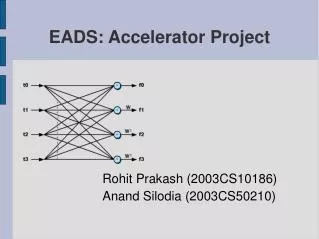
FFT Accelerator Project Rohit Prakash (2003CS10186) Anand Silodia (2003CS50210) 14th September, 2007 Supervisors : Dr. Kolin Paul Prof. M. Balakrishnan
Overview • Objective • To work out strategies for implementing efficient FFT kernel on multiprocessors and FPGA • To identify the bottlenecks
Previous Work (single processor software implementation) • Examined 3 FFT algorithms – • Radix-4 • Radix-16 • Radix-8 • Compared them with FFTW • Analysed these on the following parameters • Execution Time • Number of Complex calculations • Memory references • Vectorized the code with gcc
Previous Work : Inference • For smaller input sizes, cache misses are greatest for radix-16 (there’s a linear increase in misses from radix-4 to radix-16) • But for large input sizes, (>= 4096), the number of cache misses in radix-8 is the lowest. • Due to OOP, Complex (object) creation takes the maximum amount of Clock-ticks • Apart from that, the maximum time is taken by complex multiplications, followed by complex additions and complex subtractions
Hardware implemetation : performance issues • Circuit area • Power consumption • Speed
Algorithms : Cooley Tukey • Pros: • Because the Cooley-Tukey algorithm breaks the DFT into smaller DFTs, it can be combined arbitrarily with any other algorithm for the DFT. • Cons: • Much hardware required (16-point fft : 176 add and 72 multiply operations )
Algorithms : Winograd • Pros: • Designed to minimize the number of multiplies • Much less hardware than Cooley Tukey required (16-point fft :74 add and 18 multiply operations ) • Cons: • Highly irregular addressing sequence, which makes it very inefficient to perform with a microprocessor • awkward to factor for input sizes greater than 16
Guidelines for a suitable algorithm • Construct larger FFTs from small 4-, 8-, and 16-point FFT kernels • These smaller kernels can be Winograd • 8 point FFT is a very special case, as the multiplication can be completely replaced by addition and bit-shift operations • 16 point FFT can itself be decomposed into 4-point or 2- and 8-point FFTs
Multiprocessor FFT : Distributing Butterflies Input Distributing the butterflies on different processors would involve more IPC Output
Distributing Input Space Input Distributing the input space on different processors would involve less IPC Output
Bandwidth Measurement Data send between Abhogi and saveri at 2pm (avg. 5.4MBps)
Bandwidth Measurement Data send between jaunpuri and saveri at 11pm (avg. 5.6MBps)
Assumptions • Let TN denote the time taken to compute the FFT of input size N • Let the network bandwidth be B (bytes/sec) • Let the number of processors be p • Let the time taken to combine two N-point FFTs be KN
4 processor model Processor1 Input : N points transfer Processor1 Processor2 (N/2) points (N/2) points transfer transfer Processor1 Processor3 Processor2 Processor4 (N/4) pts (N/4) pts (N/4) pts (N/4) pts Processor4 Processor1 Processor3 Processor2 FFT(N/4) FFT(N/4) FFT(N/4) FFT(N/4) transfer transfer Processor1 Processor2 Combine Combine transfer Processor1 Combine
Pipelined structure Send(2) P4 Recv(1) FFT(N/4) Send(1) Recv(1) FFT(N/4) P3 Recv(3) Combine Send(1) Recv(1) Send(4) FFT(N/4) P2 Recv(1) Recv(1) Combine Send(2) Send(3) FFT(N/4) Combine P1 (KN/2B) (N/2B) (N/2B) (N/4B) (TN/4) (N/4B) (KN/4B) The Execution time : 2((N/2B) + (N/4B)) + (TN/4) + (KN/2B) = (3N/2B) + (TN/4) + (KN/2B)
Generalizing this • For p processors, the total execution time is : (TN/p) + (1 – 1/p)(2N/B + KN)
Further Work • Multiprocessor Implementation • Implement the above model and validate it • Hardware Implementation • Pipelining • Best utilization of the FPGA resources
References • http://www.embedded.com/columns/technicalinsights/199203914?_requestid=265790 • Hugget,Maharatna,Paul On the implementation of 128-pt FFT/IFFT for High-Performance WPAN • Michael J. Quinn, Parallel Programming in C with MPI and OpenMP