Download

1 / 65
650 likes | 754 Views
Explore the impact of fluid and solid installations on temperature sensors, considering heat transfer mechanisms and environmental factors. The chapter delves into combined heat transfer equations, including convection, radiation, and conduction. Detailed models and calculations are provided to enhance understanding.

E N D
“… the key to obtaining accurate gas temperature measurements from thermocouples is an understanding of the behavior of a bare wire thermocouple in response to its environment … radiation shields and stagnation tubes do not change a junction's sensitivity to its environment, they change its environment ...” Robert J. Moffat (1961)
In this chapter we consider separately installations in fluids and installations in solids as they affect the temperature sensor. In fluid applications, the sensor faces a complex heat transfer effect [1]-[7]. Convective heat transfer between fluid and sensor is balanced against radiative heat transfer between fluid, its enclosing walls, and the sensor, and simultaneously against conductive heat transfer between sensor and its supports. In surface applications, on the other hand, radiation and convection are assumed to affect sensor and surface roughly alike; thus conduction between sensor and its supports becomes the dominant mode of heat transfer to consider. Only secondarily must the convection effects between sensor supports and the ambient fluid be considered.
12.1 Combined Heat Transfer Equations for Fluid Installations For a physical model, consider a gas flowing in an enclosure into which is immersed a temperature sensor and its support (hereafter referred to simply as the sensor). To be specific let Tgas > Tsensor > Twall, although in a numerical case consideration of algebraic signs will allow variations in this restriction. The temperature sensor can receive heat by convection and radiation.
It can lose heat by conduction and radiation. The modes and quantities of heat transfer involved are affected by boundary conditions, gas properties, the thermodynamic state of the gas, and by the nature of the directed motion of the gas. A model of the problem to be examined is represented schematically in Figure 12.1. For a differential element of the sensor (see Figure 12.2), we can write a general heat balance expressing the conservation of thermal energy as
(12.1) dqc=dqr+(dqk/dx)dx where the subscripts have the following meanings: c = convection, r = radiation, and k = conduction. Thus our first job is to determine reasonable expressions for the various terms in (12.1). Convection Heat will be transferred to the sensor from the moving gas by forced convection. This phenomenon has been described by Newton’s cooling equation as (12.2) dqc=hcdAc(Ts-Tx)
where Ts is the static temperature of the gas, and Tx is the temperature of a differential element of the sensor. If the gas moves with an appreciable velocity, however, the temperature even an adiabatic sensor attains will not be the static temperature of the gas (see Chapter 11). Instead, the thermally isolated sensor will sense the adiabatic temperature of the gas, which can be defined in terms of (11.22) as
(12.3) where cp must be considered constant over the temperature range (Tadi-Ts). Thus it is clear that the modified Newton cooling equation to use in the heat balance of (12.1) is (12.4) The temperature distribution through the gas surrounding the sensor call be visualized as in Figure 12.3. The two coefficients of (12.4), hc and R, are discussed at greater length in Section 12.3.
Radiation There will be an interchange of radiant energy between the sensor, the gas, and the enclosing walls. For a black body, this phenomenon is described by the Stefan-Boltzmann radiation equation SENSOR EMISSION. The sensor will radiate energy according to its absolute temperature, as indicated by (12.5), modified, however, by the emissivity of the sensor, which accounts for its non-black body characteristics. Some of this energy will be absorbed by the gas and the remainder by the enclosing walls; that is, (12.5) (12.6)
But this is not the complete story. There are reflections (radiant inter-changes) between the gas and the solid gray body (the sensor) that must be considered, Effects of these reflections are included by adjusting the sensor emissivity as recommended by McAdams [8] and by Grober [9]; thus (12.7) where αg,x signifies absorptivity of the gas, to be evaluated at the sensor temperature.
For the sensor emission absorbed by the enclosing walls we have (12.8) When (12.7) and (12.8) are combined according to (12.6), we have (12.9) where Equation 12.9 represents the net rate of radiant heat transfer from the sensor.
GAS EMISSION. The gas will radiate energy according to its absolute temperature and its emissivity. The sensor will absorb some fraction of this energy incident on its surface. where єg,g signifies emissivity of the gas, to be evaluated at the gas temperature. By Kirchhoff’s law for solid bodies, αx may be replaced by єx; and again considering the reflections between the fluid and the sensor, we replace єx with (єx +1)/2 to obtain (12.10) (12.11)
WALL EMISSION. The enclosing walls will radiate according to their absolute temperature only, considering such enclosures to be black. However, the gas intercepts and absorbs some of the radiant energy emitted by the walls so that the net radiation received by the sensor from the walls is whereαg,w signifies absorptivity of the gas, to be evaluated at the wall temperature (12.12)
NET SENSOR EMISSION. By combining (12.9), (12.11), and (12.12), we obtain the expression for the net emission from the sensor by radiation, as required by the heat balance of (12.1). (12.13) For convenience (12.13) also can be expressed in terms of a radiation coefficient as (12.14) patterned after Newton’s cooling law, where (12.15)
(12.16) The coefficients hr and є’ are discussed further in Section 12.3. Conduction Heat will be transferred from the tip of the sensor (in the gas) to its base (at the wall) by means of conduction. This phenomenon is described by Fourier’s conduction equation (12.17) For an element of the sensor in the steady state (i.e., for the case of zero heat storage), the one-dimensional expression for the net conductive heat transfer, as required by the heat balance of equation (12.1), is
(12.18) The Heat Balance When (12.4), (12.14), and (12.18) are combined according to (12.1), we obtain (12.19)
12.2 Solutions to Combined Heat Transfer Equation Equation 12.19 is a second-order, first-degree, nonlinear differential equation, and as such has no known closed-form solution. It is nonlinear because the coefficients a2 and a3 are both functions of the dependent variable Tx. The offender in both cases is the radiation coefficient hr. There are at least three approaches to a solution of (12.19). Tip Solution Here all conduction effects are neglected, and (12.19) reduces to (12.20) This solution leads to a sensor tip temperature that is usually too high, since any conduction tends to reduce Ttip.
Overall Linearization Here hr, is based on an average Tx, justified by noting that (Tadi - Tw) << Tw in any practical problem. Thus for specifying the radiation coefficient only, we can approximate Tx, which is bounded by Tadi and Tw, by Tadi, Tw, or its average value (12.21) If, in addition, a right circular cylinder is assumed for the geometry of the sensor and support, the area dependence on x is removed. Under these conditions (12.19) is linearized, the coefficients a1, a2, and a3 are constants, and the closed solution is (12.22)
(12.23) This solution leads to quick, approximate answers for the case in which the gas can be considered transparent to radiation (i.e., for єg≈0), but, in general, overall linearization leads to unreliable results. Stepwise Linearization Here the solution is based on dividing the sensor and its support, lengthwise, into a number of elements, as indicated in Figure 12.4. The temperature Tx at the center of each element is taken to represent the temperature of that entire element. The number of lengthwise divisions can be made as large as desired to enhance the finite difference approximation to the nonlinear equation (12.19).
Three heat balance equations will describe the heat transfer completely through the model of Figure 12.4. TIP ELEMENT. The heat balance for element 1 is hc(Ac,0+Ac,1)(Tadi-T1)=hr,1(Ar,0+Ar,1)(T1-Tw)+kAk,1(T1-T2)/Δx From which we obtain T2=T1-(Ac,0+Ac,1) Δx/kAk,1[hcTadi-(hc+hr,1)T1+Hr,1Tw] INTERNAL ELEMENT. The heat balance for any internal element is qc,x+qk,x-1=qr,x+qk,x hcAc,x(Tadi-Tx)+kAk,x-1(Tx-1-Tx)/Δx =hr,xAr,x(Tx-Tw)+kAk,x(Tx-Tx+1)/ Δx
From which we obtain Tx+1=(1+Ak,x-1/Ak,x)Tx-(Ak,x-1/Ak,x)Tx-1-(Ac,x/Ak,x)(Δx/k)[hcTadi-(hc+hr,x)Tx+hr,xTw] (12.25) BASE ELEMENT. The heat balance for element N is qc,N+qk,N-1=qr,N+qk,N hcAc,N(Tadi-TN)+kAk,N-1(TN-1-TN)/Δx=hr,NAr,N(TN-Tw)+kAk,N(TN-Tw)/(Δx/2) From which we obtain where T’w is the calculated value of the enclosing wall temperature. Tw=(1+Ak,N-1/2Ak.N)TN-(Ak,N-1/2Ak,N)TN-1-ΔxAc,N/2kAk,N[hcTadi-(hc+hr,N)TN+hr,NTN] (12.26)
AREA CALCULATIONS. For convection and radiation calculations, it is the surface area of the sensor that is required. Considering a right circular cylinder, we have
For conduction calculations it is the cross-sectional area of the sensor that is required. Again for a right circular cyclinder we have (12.28) SOLUTION METHDO. An initial T1 is assumed (Tadi is a good first choice), and all other temperatures (T2, T3, ..., TN, and T’w) are obtained according to (12.24), (12.25) , and (12.26). The calculated wall temperature T’w is compared to the given wall temperature Tw, and adjustments in T1 are made for a second try. Iteration schemes (such as Newton’s method) rapidly lead to a unique solution for the steady-state temperature distribution throughout the sensor-support combination [10].
Comparison of the Methods The tip solution, in which conduction effects are neglected, leads to a sensor temperature that is always too high. The overall linearized solution is sometimes adequate (when єg is small), leads at times to sensor temperatures that are higher than the tip solution (whenєg≈0.5), and sometimes yields imaginary solutions (when єg≈1), in which case the ratio exceeds 1. Of course the stepwise linearized solution represents the most reliable solution of the three.
Trend Curves Because of the complex relationships between the many variables involved in the heat transfer analysis, it is easy to lose track of the physical effects of the controlling variables. In an effort to give a clearer picture of these effects, trend curves are presented in Figure 12.5 for a particular practical problem. In Figure 12.5a, note the highly beneficial effect of ensuring a substantial convective film coefficient over the thermometer well. In Figure 12.5b, the less dramatic effect of well thermal conductivity is seen. In Figure 12.5c, the importance of fluid and well emissivity is shown;
Note the insulating effect the fluid emissivity has on the thermometer well, simplifying the temperature measuring problem in steam, for example, in Figure 12.5d, the importance of insulating the enclosing walls, at least in the vicinity of the thermometer well, is seen.
Graphical Solution In Figure 12.6, a summary curve of many problems solved by the step linearized method (based on 20 steps) is given. The coordinates are the parameters of (12.22) and (12.23), that is, of the overall linearized solution. Because the actual problem is nonlinear, no exact graphical solution is possible. Even under the extremes of all the variables, however, as noted in Figure 12.6, the limits of uncertainty that attend the summary curve are relatively narrow. Thus some useful information concerning a given sensor installation can be obtained rapidly from Figure 12.6, as illustrated in several examples to follow.
12.3 Some Useful Heat Transfer Coefficients Often we must estimate a heat transfer coefficient as an item of secondary importance in a particular job [11]. A case in point is the requirement of obtaining the coefficients hc, α, and hr, in the equations of Section 12.2. There is such a confusing array of coefficients, exponents, and equations available in the various texts (see for example, Table 12.1) that it is believed best to present satisfactory values in graphical form for quick, ready estimates of these heat transfer coefficients.
Forced Convection Film Coefficients The dimensional analysis that , for forced convection , yields an expression of the form (12.29)
is well known, and advantages of the use of (12.29) in correlating large amounts of data for many different fluids are obvious [12]-[15]. The convective film coefficient hc, however, is often desired, and this requires an evaluation of the Reynolds number and then an arithmetic operation to obtain hc from the Nusselt number and the Prandtl number To simplify the procedure, the following is suggested. From (12.29) (12.30) Equation 12.30 can be rearranged to give (12.31)
Thus through the term in parentheses the film coefficient is seen to be a function of the thermodynamic state of the fluid. If a particular reference state is chosen for a particular fluid (e.g., 500 psi, 500℉ steam), a unique family of curves can be plotted in terms of hc = f(G, D). This has been done for appropriate values of a, b, and c as reported in the literature for (a) forced convection inside cylinders (see Figure 12.7); and (b) for forced convection across single cylinders (see Figures 12.5 and 12.9). To obtain the actual film coefficient hc for any fluid at any state, it is necessary only to multiply the plotted reference value of h’c by the ratio
(12.32) Correction curves representing this ratio for steam and air are given in Figures 12.10 through 12.12. These curves are required to account for variations in the thermodynamic state properties μ, k, cp.
Recovery Factor In Section 11.7 the recovery factor was discussed at some length. Briefly, there are several recovery factors to choose from. The frictional recovery factor r, based on the local adiabatic temperature, remains constant around the periphery of a cylinder. This convenient-to-use recovery factor is identical to the flat-plate recovery factors of (11.19) and (11.21). Another recovery factor is based on the undisturbed free stream velocity, the static temperature, and the mean adiabatic temperature. This is the correct recovery factor to use, but unfortunately it varies with the Mach number, and no systematic correlation exists.
However, noting that its value for air varies from 0.55 to 0.82, which is similar to the Prl/2 evaluation, and considering the inherent difficulties in the use of this mean-free r, we recommend for analysis the constant valued local rs, as defined by (11.19) and (11.21). This simplification tends to introduce a slightly greater rate of convective heat transfer to the sensor than actually exists and leads in turn to uncertainties that are on the optimistic side.
Radiation Coefficients The coefficients hrand є’ of (12.15) and (12.16) also can be represented as the ratio hr/’ in convenient graphical form, as indicated in Figure 12.13. In view of the scarcity of information on gaseous emissivity, it is suggested that advantage be taken of the simplification єg,x= єg,g = єg,w. This, together with the approximations that F of (12.9) equals l, leads to a more manageable form of (12.16), namely, (12.33)
12.4 Fluid Applications and Examples Several examples are given to illustrate the use of the graphical heat transfer coefficients in conjunction with the various combined heat transfer analyses toward solutions to typical fluid installations. Example 1. Tip Solution (involving no Conduction). Given that a spherical sensor of surface area = 0.8 in.2, disk area = 0.2 in.2, and emissivity = 1 is installed in a duct of radius 2 in. and length 6 ft, the sensor indicates 250℉ when the duct wall is at 200℉, and the convective heat transfer coefficient is 20 Btu/h-ft2-℉. Find the gas temperature. Solution (based on use of a radiation coefficient)
qc=qr hcA(Tgas-Tsensor)=hrAsurface(Tsensor-Twall) Tgas=Tsensor+(Tsensor-Twall)hr/hc in agreement with (12.20). Now from Figure 12.13, hr/ε=f(Tsensor,Twall)=f(250℉,200℉)=2.3 From (12.16) є’ = 1 if the walls and sensor are considered to be black bodies (єw= єx = 1), and if the gas is assumed to be transparent to radiation (єg= 0 ). Thus Tgas=250+(250-200)2.3/20=255.7℉ Example 2. Same as Example 1 except the Solution is now based on use of form and emissivity factors,
qc=qr hcA(Tgas-Tsensor)=FεFAσA(Tsensor4-Twall4) When the form factor FA is given according to Schenck [14] as FA=4L/(L2+R2)1/2(Adisk/Asurface)sensor= 6/(36+1/36)1/2=1 and the emissivity factor is taken as unity, the result is Tgas=Tsensor+σ(Tsensor4-Twall4)/hc Note that it is the difference in fourth-power absolute temperatures that must be used in this form of the radiation heat transfer equation. Thus Tgas=250+0.174(7.14-6.64)/20=255.6℉
We see that under the same conditions the two solutions agree within close limits. Thermometer Well Solutions Such problems resolve to the following. Given the installation details of a thermometer well, find whether the installation is satisfactory. The steps required are: 1. Remove area dependence on immersion length by approximating the given well by a right circular cylinder of the same surface area. 2. Determine the pertinent heat transfer coefficients. 3. Determine the value of (12.34)
where L = length of immersed portion of thermometer well, d = bore diameter of the well, D = outside diameter of the well. 4. If X' ≤ 20, enter Figure 12.6 with X=(hc+hr)DL2/k(D2-d2) where a3 is defined under (12.19). Now compute either Ttip or Tadi, whichever is unknown, accounting to the following: Ttip=YTwall+(1-Y)(hcTadi+hrTwall)/(hc+hr) Tadi=(hc+hr)(Ttip-YTwall)/hc(1-Y)-hrTwall/hc
On the basis of the difference between Ttip and Tadi, the worth of the installation can be judged. 5. If X' > 20, it means that conduction effects are negligible. Thus (12.36) or (12.37) are solved for Ttip or Tadi by setting Y = 0. Example 3. Air flows at a rate of 1 lb/sec at a pressure of 2 atmospheres in an uninsulated 6-in. pipe. The indicated well tip temperature is 200℉, and the indicated enclosing wall temperature is 180℉. The cylindrical well has a 3-in. immersion, 1/2in. OD, 1/8in. ID, k = 20 Btu/h-ft-℉,єwell = 0.9, єfluid = 0 (i.e., transparent). The installation is to yield fluid temperature to ±1℉.
Solution G=w/A=4×4/л=5.093lb/sec-ft2 from Figure 12.8 (low Reynolds number), from Figure 12.10 (low Reynolds number), hc=50×0.53=26.50Btu/h-ft2-℉ from Figure 12.13, by (12.16), hr=0.9×1.9=1.71Btu/h-ft2-℉ By (12.34)