Download
1 / 26
260 likes | 420 Views
Presented at the: Australasian Forest & Wood Products Conferences: Residues to Revenues. Rotorua, October 12-13 and Melbourne, October 17-18, 2005. Quantifying the availability and volume of the forest resides resource. B.Hock, P.Nielsen, S.Grigolato, J.Firth, B.Moeller, T.Evanson.

E N D
Presented at the: Australasian Forest & Wood Products Conferences: Residues to Revenues. Rotorua, October 12-13 and Melbourne, October 17-18, 2005. Quantifying the availability and volume of the forest resides resource B.Hock, P.Nielsen, S.Grigolato, J.Firth, B.Moeller, T.Evanson Scion, Rotorua, New Zealand Dept of Land and Agricultural and Forest Systems, University of Padua, Italy Dept of Development and Planning, Aalborg University, Denmark
Logging residues for energy production Energy prices are increasing Interest is growing in the use of in-forest residues as a sustainable energy resource • Consider woody biofuel as a forest product • Assess the volume available • Optimise the logistic of the supply chain • Minimise the supply cost
Biomass supply from forest plantations Two models are being developed • National availability and cost supply model • Within-forest ” ” ” ” ”
National availability and cost supply model Model overview The location of forests, the transportation network, possible cogen plant locations and other spatial issues are mapped. The information is analysed within raster GIS. Techniques include cell-to-cell functions, neighborhood statistics and zonal geometry. The results are intensity maps or distributions of site-specific costs.
National availability and cost supply model Calculating the transport cost • The accumulated travel distance from a point location determines the transportation costs along the road network to that point. • This example visualizes the cost of transportation across a region.
National availability and cost supply model Costs of biomass at site • The site-specific amount and cost of biomass are calculated by overlaying in-forest residues and transport costs. • The result is a distribution of biomass amounts and costs, which is unique for each location relative to a planned bioenergy plant.
Within forest availability and cost supply model A model was developed in collaboration with Carter Holt HarveyForests Ltd. The case study was based on the Kinleith Forest, in the North Island of New Zealand, complimented by National Exotic Forest Description (NEFD) regional yield tables
Biofuel as a product: some issues Logging residues are unevenly distributed geographically and in time Volume of residues at landings is influenced by the characteristics of the logging operation (eg. harvesting methods, equipment capacity, terrain characteristics) Extraction of residues is affected by road types and density
The within-forest chain Volume at harvest Residue at landings Transportation of residue to hogger Chipping by hogger Transportation of chips to cogen Volume and cost at cogen plant
Methodology The within-forest availability and cost supply model The components: Calculate potential amount of logging residue Assign logging residue to landings Select hogger site locations Determine transportationnetwork Minimise overall costs
Logging residue availability Investigate variables that affect availability forest stand data topography Forest Database Approximate the volume of logging residue for the next 17 years. NEFD Database forest productivity data
Logging residue availability Forest stand data calculation Kinleith Database Silvicultural Regime • analysis • only radiata pine considered Area • year of establishment • tending history • proposed felling year NEFD Database Total Recoverable Volume (TRV) • import yield tables to GIS • calculate block area • evaluate the TRV for each block • determine the logging residue for each block
Logging residue availability TRV m3/ha Residue calculation As percentage of TRV (Depends on logging method) Logging residues Volume m3/ha Drying period 1 year Volume (m3) * 0.75 t/m3 = weight (tonnes) Logging residues Weight tonne/ha
Logging residue availability Results Total Recoverable Volume (m3/year) Yearly average: 943 000 m3 Logging residue availability (tonnes/year) Yearly average: 21 500 - 28 200 tonnes Yearly average per hectare: 0.6 tonnes/ha - 0.8 tonnes/ha
Logging residue availability Results The graph shows how availability varies over time. For example, there are two periods when supply falls below 10,000 tonnes per year.
Assigning logging residue to landings • To calculate logging residue at each landing: • locate landings (12 700) • define the catchment area for each landing • overlay the logging residue • sum the logging residue for each landing • repeat for each year
Assigning logging residue to landings Location of landings with assigned residues 2006 2007 2008 Residues (red dots) vary over time and across the forest
Location of hogger sites GIS – based analysis Reclassify roads according to their carrying capacity
Location of hogger sites Selection criteria: • Must be associated with roads suitable for chip trucks • Must have a minimum area of 5000 m2
Location of hogger sites Superskid sites - 15 Superskid sites - 40 Selection criteria • Must be no closer than 20km to adjacent hogger sites
Transportation network • Network analysis to determine the minimum cost route between each landing and the hogger sites • Similarly for the routes between hogger sites and cogen plant
Minimum cost calculations • Define variables: • Maximum distance between landing and hogger site • Minimum residues at landing • Run minimum cost calculation Insert data Define scenarios Perform calculation results
legend Results Variables: maximum distance 8000 m – 9000 m residue at landing >0 in intervals of 12.5 tonne
Conclusions • the availability of residue depends not only on volume, but also on the transportation cost to the power plant • a large number of variables need to be considered including drying, in–forest logging distribution, transport and chipping techniques • GIS based models are effective tools for Decision Support Systems (DSS)