Download
1 / 117
1.17k likes | 1.18k Views
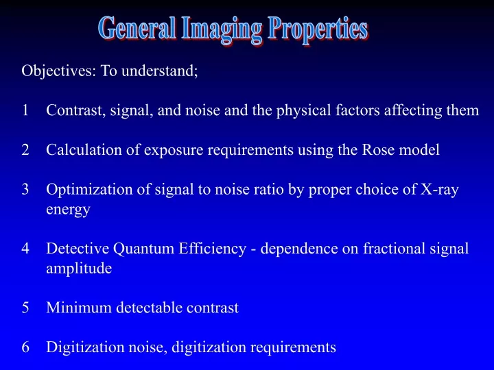
General Imaging Properties. Objectives: To understand; 1 Contrast, signal, and noise and the physical factors affecting them Calculation of exposure requirements using the Rose model 3 Optimization of signal to noise ratio by proper choice of X-ray energy

E N D
General Imaging Properties • Objectives: To understand; • 1 Contrast, signal, and noise and the physical factors affecting them • Calculation of exposure requirements using the Rose model • 3 Optimization of signal to noise ratio by proper choice of X-ray • energy • 4 Detective Quantum Efficiency - dependence on fractional signal amplitude • 5 Minimum detectable contrast • 6 Digitization noise, digitization requirements
Imaging systems are characterized by: 1. The ability to detect small attenuation changes, i.e., low contrast, faint objects. This increases as signal increases and as noise decreases. Contrast Resolution 2. The ability to see small objects, fine detail. Increases as the point spread function gets narrower. Spatial Resolution 3. The ability to stop motion and to sample motion. Increases as the exposure time decreases and the sampling rate increases. Temporal Resolution
This section addresses the factors which contribute to contrast resolution. These generally relate to overall system signal to noise ratio and the various factors affecting this quantity. Consider the differential attenuation due to some object as shown in Figure 1 No N2 N1
Subject contrast is defined as C = (N1 - N2) / N1 (1) assuming no scatter is detected. This may also be defined in terms of intensity. For monoenergetic beams the two definitions are equivalent. For polyenergetic beams the contrast would be somewhat different for the two definitions. In this discussion we will work with the definition in terms of fluence since we will be discussing numbers of x-rays.
Christensen defines C = N2 / N1. Another definition which is sometimes used is C = (N1 - N2) / ( N1 + N2) You can use any of these but you must be consistent in the derivation of results.
C =( N1 - N2)/ N approaches 0 as N1 approaches N2, and approaches 1 as N2 approaches 0. However it is defined, it refers to the difference between an object and its surroundings.
When these fluences (or intensities) are detected by a detector a signal is generated, for example, video signal or optical density. Refering to Figure 2, No Object area A Detector resolution element of area a N2 N1
the input signal S observed by each detector element a is given by S = Na The size of the detector element a is determined by whatever defines the resolution of the system, for example a picture element ( pixel ) in a digital image, or the point spread function in a film image. Perception of an object in an image is dependent upon the differential signal S representing the difference between the detected signal, integrated over the object size A, and a similar area in the region surrounding the object defined by S = N1A - N2A = (N1 -N2)A {2}
Whether this differential signal is perceptible depends on the degree of fluctuation on the signal in the area in the immediate vicinity of the object. These fluctuations, which may be due to a variety of causes are called noise. Noise = undesirable signal = n
Noise masks small signals and, along with the differential signal, determines the contrast resolution of the system. The noise relevant to the task of object detection is the average noise over an area equal to the object size. Image quality is often described in terms of signal to noise ratio. S / n = SNR ( signal to noise ratio)
The differential signal divided by the noise is also referred to as signal to noise ratio in some contexts. We will refer to this as differential signal to noise ratio. S / n = SNR ( differential SNR ) This is also sometimes referred to as contrast to noise ratio. We will not use this term since it is somewhat confusing in view of our definition of contrast as S/S.
What determines differential signal and noise? SignalNoise subject Contrast quantum noise kVp system noise filtration anatomical noise object observer noise scatter artifacts detector display
Ideal Systems - Exposure Requirements Consider exposure requirements for contrast and spatial resolution in an IDEAL SYSTEM - i.e. one in which all noise due only to quantum noise, ( statistical fluctuations in the number of transmitted x-rays). X-ray noise is described by a Poisson distribution as shown in Figure 3. n = (N1A)1/2 = N n Probability of #x-rays in area A N1 Fluence N
Calculation of Image Signal to Noise Ratio - Small Contrast The differential signal is given by equation 2 as S = ( N1 - N2 ) A For very small contrasts and (3)
Therefore we can write S =NCA (4) The noise is given by (5) so (6)
Calculation of Required Exposure - Rose Model According to equation 6, the detected fluence is related to the s/n by (7) The detected fluence is related to the incident fluence N0 by the transmission factor T as N = N0 T (8) (For non-ideal systems the detection efficiency of the detector would also multiply the transmission factor in the above equation)
Therefore the incident fluence is related to the imageSNR by (9)
The ROSE MODEL is a model which assumes that the statistical fluctuations calculated above are the only determinant of perception. The effects of edge gradients, which are known to be important, are not considered. The Rose model states that small contrasts will be visualized when SNR = 3 - 5
We can use the Rose model to obtain approximate estimates of required exposure. We can illustrate the Rose model using a raindrop analogy. Suppose you had a marble and a basketball on your driveway as shown in Figure 4. Figure 4
After a small amount of rain, if you removed these objects, you could detect the presence of the basketball, but not that of the marble. This is illustrated in Figure 5. Figure 5
As more rain falls, and the average spacing of the raindrops becomes smaller than the marble, you can begin to see the dry spot under the marble when it is removed. This is illustrated in Figure 6 where we have only included the region around the marble. Figure 6
A lot more rain is required to define the marble than the basketball. A higher fluence (exposure) is needed to visualize small objects. So for an ideal system, No is proportional to 1/ A, 1 / C2, 1/ T, and ( s / n )2.
DEPENDENCE OF IMAGE QUALITYON X-RAY EXPOSURE 0.400 mR 0.025 mR Kruger and Reiderer Basic Concepts of Digital Subtraction Angiography p 80-81
Example: Intravenous Angiography For some time after the initial introduction of digital subtraction angiography techniques radiologists investigated the possibility of obtaining angiograms using intra-venous injections of contrast material, usually into a vein in the arm, but sometimes using a catheter placed in the superior vena cava or right atrium. Although considered less invasive than intra-arterial catheter placement, this technique required high system contrast sensitivity because of the fact that the contrast was diluted by a factor of twenty or so, depending on cardiac output, before reaching the arteries of interest.
Suppose we have low iodine contrast in a vessel following intravenous injection and we want to detect 1 mm long narrowing of the vessel as shown in Figure 7. 1 mm 1 mm N1 N2
Suppose: I = 5 mgm/cm3 iodine density at the artery after iv injection t = 1 gm/cm3 tissue density t = 20 cm µtissue = µt = 0.25 cm2 / gm µiodine = µI =15 cm2/gm Keff = 35 keV
Then C = (N1 - N2) / N1 = (e-µt * 2 0 - e-µt*20- µI ∆tI) / (e-µt* 20) = 1 - e - µI ∆tI ~ 1 - ( 1 - µI ∆tI .... )
Therefore, in general, for small contrasts (10) Plugging in, we get C = µI ∆tI = µI pl ∆xI = 15 cm2/gm* .005 gm/cm3* .1 cm = .0075 The transmission factor is
Remembering that 1R ≈ 2x10¹⁰ photons/cm2 at 35 keV we get a required incident exposure of E0 ~ .12 R
This is the exposure required to image the 1mm length of a contrast filled vessel. This should also be approximately the exposure required to see a total stenosis with a length approximately equal to the vessel diameter. This shows that exposure is not only related to contrast resolution, but also can limit spatial resolution, i.e., in order to see something very small (of low contrast), a large exposure is required.
For example, what if ∆tI decreases to 0.1 mm, down by a factor of ten? Then contrast decreases by a factor of ten to 0.0075, area goes down by ten, assuming we are still looking at a 1mm length, and T stays the same since it is dominated by the tissue transmission. Then N0 = 2.39 x 109 x 102 x 10 = 2.39 x 10¹² E0 = 119 R !
The effect of increasing the number of quanta in an image are illustrated in Figure 8 for the case of light photons. This is from Rose’s book called Vision.
4 3 ROSE W0MAN 3 • 10 1.2 • 10 5 4 9.3 • 10 7.6 • 10 7 5 2.8 • 10 3.6 • 10
An illustration of the same principle using x-rays is illustrated in Figure 9. Figure 9A shows an attempt to image the arteries in the head using an intravenous injection. For this image there was a malfunction of the exposure regulation circuitry and the exposure was approximately a factor of 100 less than anticipated. Figure 9B shows the examination repeated with the correct exposure. The increase in image quality is evident. A B Figure 9
We can use the Rose model to calculate optimal beam energies for various situations. Again, we assume quantum statistical noise dominates image noise. We will try to determine the optimum x-ray energy for a particular imaging problem. CASE I: Small tissue thickness t on a larger tissue thickness t (gm/cm2) as shown in Figure 10. Ideal Systems - Spectral optimization N0 t ∆t N1 N2
From equation 9 No ≈ (s /n )2 / C2AT so for fixed s /n and A where µtis the effective attenuation coefficient over distance t, ignoring the details of beam hardening for now.
but Therefore,
Now we can find the beam energy which minimizes exposure which is No using the usual calculus max / min procedure of setting the first derivative to zero. No (e µtt) / µt2(11) (dNo) / (dµt) = (teµtt) / (µt2) + (-2eµt t) / (µt3) = 0 (12) which gives µt = 2 / t (13) That this is a minimum and not a maximum can be checked by looking at the second derivative.
Chest imaging: t ≈ 20 cm The attenuation coefficient associated with the optimal energy is given by the above equation as µT = 2/20 = 0.1 cm2/gm This corresponds to an effective beam energy of about 100 keV and a kVp of something like 200 depending on the filtration. Example 1
Mammography t ≈ 5 cm The same analysis results in µt = 2/5 cm2/gm Keff = 25 keV for tissue and 23 keV for fat Bear in mind that these are ideal system results. For actual mammography, where object contrast must be kept somewhat higher than the ideal to compete with addition system noise such as film grain, the optimal energies actually used are somewhat lower. Example 2
Daffodil Imaged at 5 and 20kV 5 20 Gilardoni et al. Radiology-Electromedicine
From the examples, we see that the best energy is very thickness dependent. There is a tradeoff between transmission and contrast. For large tissue thicknesses, transmission is the most important factor, i.e., it is desirable to use the highest kVp possible until the contrast is so small that it becomes comparable to the system noise. In computed tomography, with high device SNR, studies show 140 kVp to be superior to 80-120 kVp for tissue tumor detection.
Refer to Figure 10 below, with a small iodine thicknesstI substituted for the small tissue thickness t. In this case, for fixed A and tI, the required fluence is given by No ≈ (s/n)2 / (C2 1 / (C2 e-µt t)(14) CASE II: Iodine Imaging N0 t ∆t N1 N2
but since C ≈ µItI No (e+µt t) / (µI2∆tI2) (e µt t) / µI 2(15) Now we have an expression involving two attenuation coefficients, both of which are dependent upon energy. Therefore, the differentiation involved in the minimization procedure must be with respect to energy. In order to accomplish this we will have to parameterize the attenuation coefficients in terms of the energy k and fill in the appropriate terms in the expression. dN / dk = (N / µI) (dµI/dk) + N /µT)(dµT/dk) = 0 (16)
For tissue the Compton and photoelectric contributions are both ≈ 0.25 cm2/gm at 25 keV. Modeling the Compton contribution as a constant with energy and inserting the known energy dependence of the photoelectric component we get µT ≈ 0.25 [1 + (25/k)3] (17) For iodine we can make the approximation that the only significant contribution is photoelectric because of the high atomic number of iodine. Normalizing to the value of 36cm2/gm at 33 keV we get, µI ≈ 36 (33/k)3 valid for keV > 33 (18)
From these expressions for the attenuation coefficients we get (dµT / dk) = (0.25)(25)3 (-3)/(k4) (dµI)/(dk) = (36)(33)3 (-3) / k4 Inserting into equation 16, we get, dN / dk =[ e µt t (-2) / (µ3I) ](36)(33)3 (-3)/(k4) + [te µt t / µ2I] (0.25)(25)3 (-3) / (k4) = 0 Simplifying, [2(36)(33)3] / (µI) = t (0.25)(25)3
Substituting for µI gives, [2(36)(33)3] / [(36)(33)3/k3] = t (0.25)(25)3 solving for k we get, k3 = t [(0.25) / 2] (25)3 k = 25 (0.25/2)1/3 t1/3 k = 12.5 t1/3 for k > 33 keV (19)
For k < 33 keV the model does not apply. At 33 keV t = 18 cm. For t < 18 cm 33 kev will minimize the exposure. For t > 18cm the above formula predicts that the optimal energy increases away from the k-edge very slowly with thickness. For example at t = 27 cm, k =12.5(27)1/3 = 12.5(3) = 37.5 keV
This dependence is quite different from that of tissue where the optimal energy for detecting small tissue contrasts was considerably higher at the same tissue thickness, e.g. CASE I (tissue detection): t = 20 CASE II( iodine detection): k ≈ 100 keV k ≈ 34 keV