Download
1 / 34
340 likes | 379 Views
Gene Frequency and Genotypic Frequency. It refers to the relative abundance or the relative rarity of a particular gene in a population as compared to its own alleles in that that particular population.

E N D
Gene Frequency and Genotypic Frequency • It refers to the relative abundance or the relative rarity of a particular gene in a population as compared to its own alleles in that that particular population. • The frequency of a gene varies between zero and one. When the frequency of a particular gene is one, the frequency of its allele will be zero in that population. • The gene frequency is also defined as the proportion of a particular gene in the total gene pool • while genotypic frequency is defined as proportion of a genotype in the population. • If there was a herd of 100 Shorthorn cattle, with 40 red, 40 roan and 20 white individuals, the frequency of red cattle is 40% or 0.4, while roan and white have 0.4 and 0.2 frequencies, respectively.
The gene frequency can be calculated as follows:- Phenotype Red Roan White Total Genotype RR Rr rr No. 40 40 20 100 No. R 80 40 - 120 r - 40 40 80 Frequency of R gene 120/200 = 0.6 Frequency of r gene 80/200 = 0.4 Here it is assumed that the forces that change the gene frequency are absent.
Hardy-Weinberg Law • In a large random mating population, the genotypic and gene frequency will not be changed generation after generation in the absence of any external force i.e. selection, mutation or migration. • Furthermore, they follow a simple relationship (A + B)2 A2 + 2AB + B2 • For illustration, let us make a mating of a homozygous polled bull with homozygous horned cow: • P1 Polled bull horned cow • PP x pp • F1 Pp all horned
Inter se mating F2 PP Pp pp 1 2 1 Genes P (2) , P (2) p(2) p (2) • The gene frequency will be 0.5 for each gene in F1. The frequencies of two genes in F2 will be 4 P and 4 p genes, showing that the frequency of each gene is still 0.5 • and if the horned animals are discarded, there would be a total of 4 P and 2 p genes left, and the frequency of the two genes would be 0.67 and 0.33, respectively.
In a herd of 100 short horn cattle 50 are red, 40 are roan and 10 are white. What are the frequencies of red and white genes in this herd. There are 100 individuals, so there would be 200 genes red and white. Coat colour phenotype Genotype No. Of individuals No. Of (R) gene (r) gene Red RR 50 100 -- Roan Rr 40 40 40 White rr 10 -- 20 100 140 60 Calculating Gene Frequencies in a Population when No Dominance Frequency of (R) gene = 140/200 = 0.7 “r” = 60/200 = 0.3 Frequency of Red gene + frequency of white gene will be 0.7+0.3 = 1.0
The population of roan individuals can be estimated using the Hardy Weinberg law • (R+r)2 • R2 + 2Rr + r2 • What will be the probability that a sperm from the above population carrying the red gene will fertilize an egg carrying the red gene? • The probability of two or more independent events, occurring together is equal to the product of the probabilities for each event separately. • Thus the probability of a sperm and egg to fertilize to pair two red genes in the zygote is 0.7 x 0.7 = 0.49. • Similarly the probability of the sperm carry white gene to fertilize the egg carrying the white gene will be 0.30 x 0.30 = 0.09.
Similarly, the proportion of roan individuals can be calculated. • The probability of sperm carry (R) gene to fertilize an egg with (r) gene will be 0.7 x 0.3 = 0.21 and (r) sperm to (R) egg, will be 0.3 x 0.7 = 0.21. • Since the individual rR and Rr are exactly the same, so the proportion will be 0.21+0.21=0.42. So the genotypic frequency will be 0.49 (RR),0.42 (Rr) and 0.09 (rr)
Calculating Gene Frequency when Dominance is Complete • In a large random mating population, where the frequency of one of the two alleles is “a”, and the frequency of the other allele is “b”, in the next generation the offspring of three genotypes will occur in a definite ratio, at the frequencies of a2, ab, b2. i.e. • No. of homozygous dominant individuals = a2 • No. of heterozygous individuals = 2ab • No. of homozygous recessive individuals = b2 • Dwarfism in beef cattle is a recessive character; where as normal size is dominant. In a purebred herd of beef cattle, fourout of every 100 calves born are dwarfs. It is very difficult to ascertain the carrier normal animals in this population. Through the use of gene frequency concept, we can calculate the frequency of dwarf genes.
Normal DD Carrier Dd and Dwarf dd Dwarf dd = 4 i.e. 4/100 = 0.04 d2 = 0.04 D2 + 2Dd + d2 The proportion of dwarf progeny will be d2 or 0.04, and the frequency of d gene will be √d2 ═ √0.04 ═ 0.20 and the frequency of D will be 1.00 - 0.20= 0.80. The proportion of heterozygous individuals will be 2(0.80 x 0.20) = 0.32 In other words 32 out of each 100 calves produced will be heterzygotes i.e carrier of the dwarf genes.
Records indicate that approximately one black Angus out of every 200 is red instead of black. • BB Black Bb Black bb Red • Red bb = 1/200 = 0.005 • b2 = 0.005 • b = 0.07 • The frequency of red gene is √0.005 = 0.07. • Frequency of black gene will be (1- 0.07) = 0.930 in the progeny. • The expected frequency of the heterozygous black progeny from parents mated at random for the red and black colour would be 2(0.07 x 0.93), or about 13 out of each 100. • If only black parents were need for breeding, the frequency of the heterozygous black individuals would be about 13 percent.
FACTORS MODIFYING GENE FREQUENCY • The frequency of same allele may be quite different in separate populations with in a single species. • The frequency of the black coat colour gene is zero in Hereford Cattle but very high in Angus Cattle. • Why does this variation occur? There are many factors that change the gene frequency. There are four major factors responsible for such variations. • Selection, mutation, migration, random drift (chance variation, genetic drift)
Selection • This is a very important factor that may be responsible for changes in gene frequencies. • Selection has important effects on gene frequencies. • It is the only tool available to man that he can use to make permanent changes in the productivity of populations by changing the frequency of desired genes. • Selection may be defined as differential reproductive rate for certain individuals. • It means that individuals possessing certain desirable traits are caused or allowed to produce the next generation. • Thus, individuals of a certain genotype may be retained in larger numbers for breeding purposes than others. This causes an increase in the frequency of some genes and a decrease in the frequencies of others
We have herd of 100 shorthorn cows consisting of 25 red, 50 roan and 25 White. • In this herd the frequency of each gene i.e. (R) and (r) will be 0.5. • The former decided to cull and sell all white individuals. • By this we will have 25 red and 50 roan individuals. The frequency of red (R) genes will be 0.667 and frequency of (r) white genes will reduce to 0.333. • RR Rr R r • 25 50 RR 50 - Rr 50 50 100 50 • Frequency of R = 100/150 = 0.667 • r. = 50/150 = 0.333 • By culling all roan (Rr) and White rr the frequency of (R) gene will be 1 and for (r) gene will be 0.
Continued • Selection can be of two types, artificial and natural. • Artificial selection is that practiced by man, whereas natural selection is done by nature in causing death of the less viable individuals. • Both types of selection have been very effective in the past when considered over a long period of time, as shown by the presence of different breeds of sheep, cattle, horses and other farm animals. • One of the main differences between breeds is that they differ in the frequencies of genes for certain traits.
Gene Mutations • This source of genetic variability proposes new genes. Mutation must be recognized for the important part it plays in providing new variation over long periods of time, permitting the population to adopt to changing environmental stress. • Mutations are generally much less important in changing gene frequency as most mutation rates are low and most mutations are harmful. • Positive and negative mutations are almost in equilibrium • They are generally recessive in nature and it makes it difficult to increase their frequency in initial selection
Migration • The introduction of new genes into a population can change gene frequency: • Widespread introductions are utilized in crop breeding, but in purebred livestock populations it is not usually a widespread importance. • Any change which migration invokes is dependent on the frequency of the gene in the immigrant population and the extent to which the immigrants are allowed to propagate, i.e. the proportion of gametes they are permitted to furnish
Chance variation or genetic drift • Changes in gene frequency also can result just from chance due to Mendelian sampling which takes place in providing the gametes which represent the gene pool for the next generation. • In large populations this chance is less important to have a change in gene frequency but in smaller populations this force do exert its impact. • Inbreeding is a potential source for change in frequency of certain genes. • Under inbreeding the population number is restricted, since matings take place within a closed herd or flock. • The smaller the population the more drastic may be the genetic drift or possible change in gene frequency due to chance, just as the smaller the inter-mating population, the more intense the rate of inbreeding
SOME STATISTICAL TOOLS COMMONLY USED IN ANIMALS PRODUCTION • Animal production is mostly concerned with populations of animals, groups of individuals that have one or many things in common, such as belonging to the same flock/herd, breed or species. • The numerical values of observations such as milk production, birth weight, weaning weight, adult weight etc. are known as variables. • Since, in quantitative inheritance, the phenotypes are not distinct and separate but exhibit a series of variations between the extremes, mathematical/statistical methods have been devised for measuring and describing populations.
Animal production is mostly concerned with populations of animals, groups of individuals that have one or many things in common, such as belonging to the same flock/herd, breed or species. • Variables: The numerical values which vary from individual to individual or the observations such as milk production, birth weight, weaning weight, adult weight etc. • Qualitative: (only can be described) like color, beauty • Quantitative (measurable) height, weight
The Mean: The first estimate used to describe a group of observations is average or mean or arithmetic mean. It is the sum of the observations divided by the number. X = X1 + X2 + X3 + X4 + ………. Xn N X = Xi / N The mean summarizes all values into a single figure that is typical of the entire set of figures in that it is intermediate among the individual values. The Range: The range is a very rough measure of the variation with in a population. It is determined by finding the lowest and the highest values within a series or group of figures. The chief disadvantages of the range as a measure of variation are that it is subject to chance fluctuations and that it becomes larger as size of the sample increases
The Variance: The degree of dispersion or variation exhibited by a population can be expressed as the average deviation or difference from the mean, ignoring signs. The range between the extremes of the population also provides some indication of variability. However, these measures do not explain well the variability in the populations. The variance is the most useful measure of variation for studying the variability in the population and is usually denoted by the symbol 2 and is defined as the average of the squared deviations of the individual measurements from the population mean. 2=(X1 - X)2 + (X2 - X)2 + (X3 - X)2 + . . . . . . .+ (Xn - X)2 n - 1 2 = ( Xi-X )2 / n –1 Since the deviations are squared, the variance is a positive value with zero as a lower limit. In case of large number of observations, there may be difficulty in calculations and a chance of error is also there, So a machine formula is used: 2 = X2 - ( X) 2 / n n - 1
XI Xi2 ( Xi-X ) ( Xi-X )2 4 16 -2 4 7 49 1 1 5 25 -1 1 8 64 2 4 6 36 0 0 30 190 0 10 Example The measurements on body weight of lambs are as under N = 5 X = 6
2 = X2 - ( X) 2 / n n - 1 2 = 190 - 900/ 5 = 190 - 180 = 2.5 4 4 One of the most useful properties of the variance is that it can be separated by a special analysis into its various component parts. Special adaptations of the analysis of variance can be used to determine the percentage of the variation in a population due to inheritance and that is due to environment. One of the most useful properties of the variance is that it can be separated by a special analysis into its various component parts i.e Analysis of variance (ANOVA). Special adaptations of the analysis of variance can be used to determine the percentage of the variation in a population due to inheritance and that is due to environment.
The Standard Deviation The standard deviation is a much more accurate measure of variation in a population than is the range, and can be used very effectively, together with the mean, to describe a population. The standard deviation is the square root of the variance. The units of variance are kilograms, centimeters squared, the units for the standard deviations are kgs or cms just as the original items were measured. (SD) = √ (X1 - X)2 + (X2 - X)2 + . . . . . . .+ (Xn - X)2 n - 1 SD () = √ Xi2 - ( Xi) 2 / n n - 1
Empirical Formula • Mean 1 = 68 % • Mean 2 = 95 % • Mean 3 = 99 % • The mean ± one S.D includes approximately 68 percent of the individuals in the population. • Mean ± 2 SDincludes 95% of the individuals of the population. • In other words, we might expect only about 5% of the population to fall outside the mean ± 2 S.D. • However, it applies only to the normal distribution
Hypothetical Example A population of 1000 cows has mean milk production per lactation as 1500 kg with a standard deviation of 100 kg. Out of this population approximately 680 cows will have the milk production ranging from 1400-1600 kg (Mean ±1 SD or 1500±100) and about 950 cows will fall within the range of 1300 – 1700 kg (Mean ± 2 SD). In other words approximately 500 cows will be producing more than 1500 kg of milk in lactation and about 160 cows will be producing more than 1600 kg of milk whereas 25 animals will be producing more that 1700 kg of milk per lactation and only 5 animals will fall in category producing more than 1800 kg of milk
The coefficient of variation & Coefficient of Correlation The coefficient of variation is another method of expressing the amount of variation within a particular population. • C.V. = S.D x 100 X • The coefficient of variation is the fraction or percentage that the standard deviation is of the mean. • One important use of this statistic is that it can be used to compare the variations of two unrelated groups. • The coefficient of correlation is referred to as “r” and gives a measure of how two variables tend to move together. • They are said to be positively correlated if they tend to move together in the same direction; that is, when one increases, the other increases, or when one decreases the other also decreases. • They are said to be negatively correlated if they tend to move in opposite directions; that is, when one increases the other decreases. Thus, the coefficient of correlation for two variables lie somewhere between zero ± 1
r = XiYi - ( Xi) . ( Yi) / n √ Xi2 - ( Xi) 2 / n . √ Yi2 - ( Yi) 2 / n Where Xi = each individual observation for variable X Yi = each individual observation for variable Y n = number of observations for each variable = the sum of all items for each variable or pair of variables.
Regression • Correlation-“r”----measures the degree of association between two variables • (no mention of independent or dependent) • Regression--“b”--- measures the amount of change in one variable (dependent) associated with a unit change in the second variable (independent) • In regression one variable is independent (cause) and the other is dependent (effect)
Regression byx= XiYi - ( Xi) . ( Yi) / n Xi2 - ( Xi) 2 / n X is independent bxy= XiYi - ( Xi) . ( Yi) / n Yi2 - ( Yi) 2 / n Y is independent The regression finds most use in predicting or estimating one variable, provided the other variable is known. Y = Y + b (Xi - X)
X = 6 Y = 16 2X = 10/4 = 2.5 2Y = 40/4 = 10.0 r = XiYi - ( Xi) . ( Yi) / n √ Xi2 - ( Xi) 2 / n . √ Yi2 - ( Yi) 2 / n r = 500 – 30 x 80/5 = 1.00 √ 190 – 900/5 . √ 1320 –6400/5
byx = XiYi - ( Xi) . ( Yi) / n Xi2 - ( Xi) 2 / n byx = 500 - 30 x 80/5= 2.0 190 – 900/5 bxy = XiYi - ( Xi) . ( Yi) / n Yi2 - ( Yi)2 / n bxy = 500 - 30 x 80/5= ½ or 0.5 1320 –6400/5 For the value of X, 7, what will be the corresponding value of Y Y = Y + b (X - X) = 16 + 2 (7- 6) = 18
r = Covariance X.Y X. Y byx = Covariance X.Y 2X. bxy = Covariance X.Y 2y.