Download
1 / 26

E N D
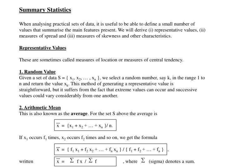
Summary StatisticsWhen analysing practical sets of data, it is useful to be able to define a small number of values that summarise the main features present. We will derive (i) representative values, (ii) measures of spread and (iii) measures of skewness and other characteristics.Representative ValuesThese are sometimes called measures of location or measures of central tendency.1. Random ValueGiven a set of data S = { x1, x2, … , xn }, we select a random number, say k, in the range 1 to n and return the value xk. This method of generating a representative value is straightforward, but it suffers from the fact that extreme values can occur and successive values could vary considerably from one another.2. Arithmetic MeanThis is also known as the average. For the set S above the average is x = {x1 + x2 + … + xn }/ n.If x1 occurs f1 times, x2 occurs f2 times and so on, we get the formula x = { f1 x1 + f2 x2 + … + fn xn } / { f1 + f2 + … + fn } ,written x = f x / f , where (sigma) denotes a sum.
Example 1. The data refers to the marks that students in a class obtained in an examination. Find the average mark for the class. The firstpoint to note is that the marks are presented as Mark Mid-Point Numberranges, so we must be careful in our of Range of Studentsinterpretation of the ranges. All the intervals xi fi fi ximust be of equal rank and their must be no gaps in the classification. In our case, we 0 - 19 10 2 20interpret the range 0 - 19 to contain marks 21 - 39 30 6 180greater than 0 and less than or equal to 20. 40 - 59 50 12 600Thus, its mid-point is 10. The other intervals 60 - 79 70 25 1750 are interpreted accordingly. 80 - 99 90 5 450 Sum - 50 3000 The arithmetic mean is x = 3000 / 50 = 60 marks. Note that if weights of size fi are suspended x1 x2 x xnfrom a metre stick at the points xi, then the average is the centre of gravity of the f1 fndistribution. Consequently, it is very sensitive f2to outlying values. Equally the population should be homogenous for the average to be meaningful. For example, if we assume that the typical height of girls in a class is less than that of boys, then the average height of all students is neither representative of the girls or the boys.
3. The ModeThis is the value in the distribution that occurs most frequently. By common agreement,it is calculated from the histogram using linear interpolation on the modal class.The various similar triangles in the diagram generate the common ratios. In our case, the mode is 60 + 13 / 33 (20) = 67.8 marks.4. The MedianThis is the middle point of the distribution. It is used heavily in educational applications. If{ x1, x2, … , xn } are the marks of students in a class, arranged in nondecreasing order, then the median is the mark of the (n + 1)/2 student.It is often calculated from the ogive or cumulative frequency diagram. In our case,the median is 60 + 5.5 / 25 (20) = 64.4 marks. Frequency 50 13 20 25 13 20 12 6 2 5 20 40 60 80 100 Cumulative Frequency 50 25.5 20 40 60 80 100
Measures of Dispersion or ScatteringExample 2. The following distribution has the same Marks Frequencyarithmetic mean as example 1, but the values are more x f fxdispersed. This illustrates the point that an average value on its own may not be adequately discribe 10 6 60statistical distributions. 30 8 240 50 6 300To devise a formula that traps the degree to which a 70 15 1050distribution is concentrated about the average, we 90 15 1350consider the deviations of the values from the average. Sums 50 3000If the distribution is concentrated around the mean, then the deviations will be small, while if the distribution is very scattered, then the deviations will be large. The average of the squares of the deviations is called the variance and this is used as a measure of dispersion. The square root of the variance is called the standard deviation and has the same units of measurement as the original values and is the preferred measure of dispersion in many applications. x6 x5 x4 x3 x2 x1 x
Variance & Standard Deviation s2 = VAR[X] = Average of the Squared Deviations =S f { Squared Deviations } / S f = Sf { xi - x } 2 / S f = S f xi 2 / S f - x 2 , called the product moment formula. s = Standard Deviation = Ö VarianceExample 1 Example 2f x f x f x2 f x f x f x22 10 20 200 6 10 60 6006 30 180 5400 8 30 240 720012 50 600 30000 6 50 300 1500025 70 1750 122500 15 70 1050 735005 90 450 40500 15 90 1350 12150050 3000 198600 50 3000 217800VAR [X] = 198600 / 50 - (60) 2 VAR [X] = 217800 / 50 - (60)2 = 372 marks2 = 756 marks2
Other Summary StatisticsSkewnessAn important attribute of a statistical distribution relates to its degree of symmetry. The word “skew” means a tail, so that distributions that have a large tail of outlying values on the right-hand-side are called positively skewed or skewed to the right. The notion of negative skewness is defined similarly. A simple formula for skewness is Skewness = ( Mean - Mode ) / Standard Deviationwhich in the case of example 1 is: Skewness = (60 - 67.8) / 19.287 = - 0.4044.Coefficient of VariationThis formula was devised to standardise the arithmetic mean so that comparisons can be drawn between different distributions.. However, it has not won universal acceptance. Coefficient of Variation = Mean / standard Deviation. Semi-Interquartile RangeJust as the median corresponds to the 0.50 point in a distribution, the quartiles Q1, Q2, Q3 correspond to the 0.25, 0.50 and 0.75 points. An alternative measure of dispersion is Semi-Interquartile Range = ( Q3 - Q1 ) / 2.Geometric MeanFor data that is growing geometrically, such as economic data with a high inflation effect, an alternative to the the arithmetic mean is preferred. It involves getting the root to the power N = S f of a product of terms Geometric Mean = NÖ x1f1 x2f2 … xkfk
Regression[Example 3.] As a motivating example, suppose we are modelling sales data over time. SALES 3 5 4 5 6 7 TIME 1990 1991 1992 1993 1994 1995We seek the straight line “Y = m X + c” that best approximates the data. By “best” in this case, we mean the line which minimizes the sum of squaresof vertical deviations of points fromthe line: SS = S ( Yi - [ mXi + c ] ) 2.Setting the partial derivatives of SS with respect to m and c to zero leads to the “normal equations” S Y = m S X + n .c , where n = # pointsS X .Y= m S X2 + c S X .Let 1990 correspond to Year 0.X.X X X.Y Y Y.Y 0 0 0 3 9 1 1 5 5 25 4 2 8 4 16 9 3 15 5 25 16 4 24 6 36 25 5 35 7 49 55 15 87 30 160 Y = m X + c Y Yi m Xi + c 0 X Xi Sales 10 5 Time 0 5
Example 3 - Workings.The normal equations are: 30 = 15 m + 6 c => 150 = 75 m + 30 c 87 = 55 m + 15 c 174 = 110 m + 30 c=> 24 = 35 m => 30 = 15 (24 / 35) + 6 c => c = 23/7Thus the regression line of Y an X is Y = (24/35) X + (23/7)and to plot the line we need two points, so X = 0 => Y = 23/7 and X = 5 => Y = (24/35) 5 + 23/7 = 47/7. It is easy to see that ( X, Y ) satisfies the normal equations, so that the regression line of Y on X passes through the “Center of Gravity” of the data. By expanding terms, we also getS( Yi - Y ) 2 = S ( Yi - [ m Xi + c ] ) 2+ S ( [ m Xi + c ] - Y ) 2Total Sum ErrorSum Regression Sumof Squares of Squares of SquaresSST = SSE + SSRIn regression, we refer to the X variable as the independentvariable and Y as the dependent variable. Y Yi mXi +C Y Y X X
CorrelationThe coefficient of determination r2 ( which takes values in the range 0 to 1) is a measure of the proportion of the total variation that is associated with the regression process: r2 = SSR/ SST = 1 - SSE / SST.The coefficient of correlation r ( which takes values in the range -1 to +1 ) is more commonly used as a measure of the degree to which a mathematical relationship exists between X and Y. It can be calculated from the formula: r = S ( X - X ) ( Y - Y )ÖS ( X - X )2 ( Y - Y ) 2 = n S X Y - S X S YÖ{ nSX 2 - ( S X ) 2 } { nSY 2 - ( S Y ) 2 }Example. In our case r = {6(87) - (15)(30)}/ Ö{ 6(55) - (15)2 } { 6(160) - (30)2 } = 0.907. r = - 1 r = 0 r = + 1
ColinearityIf the value of the correlation coefficient is greate than 0.9 or less than - 0.9, we would take this to mean that there is a mathematical relationship between the variables. This does not imply that a cause-and-effect relationship exists.Consider a country with a slowly changing population size, where a certain political party retains a relatively stable per centage of the poll in elections. Let X = Number of people that vote for the party in an election Y = Number of people that die due to a given disease in a year Z = Population size.Then, the correlation coefficient between X and Y is likely to be close to 1, indicating that there is a mathematical relationship between them (i.e.) X is a function of Z and Y is a function of Z also. It would clearly be silly to suggest that the indicence of the disease is caused by the number of people that vote for the given political party. This is known as the problem of colinearity. Spotting hidden dependencies between distributions can be difficult. Statistical experimentation can only be used to disprove hypotheses, or to lend evidence to support the view that reputed relationships between variables may be valid. Thus, the fact that we observe a high correlation coefficient between deaths due to heart failure in a given year with the number of cigarettes consumed twenty years earlier does not establish a cause-and-effect relationship. However, this result may be of value in directing biological research in a particular direction.
Overview of Probability TheoryIn statistical theory, an experiment is any operation that can be replicated infinitely often and gives rise to a set of elementary outcomes, which are deemed to be equally likely. The sample space S of the experiment is the set of all possible outcomes of the experiment. Any subset E of the sample space is called an event. We say that an event E occurs whenever any of its elements is an outcome of the experiment. The probability of occurrence of E is P {E} = Number of elementary outcomes in E Number of elementary outcomes in SThe complement E of an event E is the set of all elements that belong to S but not to E. The union of two events E1 E2 is the set of all outcomes that belong to E1 or to E2 or to both. The intersection of two events E1 E2 is the set of all events that belong to both E1 and E2.Two events are mutually exclusive if the occurrence of either precludes the occurrence of the other (i.e) their intersection is the empty set . Two events are independent if the occurrence of either is uneffected by the occurrence or nonoccurence of the other event.Theorem of Total Probability. P {E1 E2} = P{E1} + P{E2} - P{E1 E2}Proof. P{E1 E2} = (n1, 0 + n1, 2 + n0, 2) / n = (n1, 0 + n1, 2) / n + (n1, 2 + n0, 2) / n - n1, 2 / n = P{E1} + P{E2} - P{E1 E2}Corollary.If E1 and E2 are mutually exclusive, P{E1 E2} = P{E1} + P{E2} S E S n = n0, 0 + n1, 0 + n0, 2 + n1, 2 E1 E2 n1, 0 n1, 2 n0, 2 n0, 0
The probability P{E1 | E2} thatE1 occurs, given that E2 has occurred (or must occur) is called the conditional probability of E1. Note that in this case, the only possible outcomes of the experiment are confined to E2 and not to S.Theorem of Compound ProbabilityP{E1 E2} = P{E1 | E2} * P{E2}.Proof. P{E1 E2} = n1, 2 / n = {n1, 2 / (n1, 2 + n0, 2) } * { n1, 2 + n0, 2) / n} Corollary.If E1 and E2 are independent, P{E1 E2} = P{E1} * P{E2}. The ability to count the possibily outcomes in an event is crucial to calculating probabilities. By a permutation of size r of n different items, we mean an arrangement of r of the items, where the order of the arrangement is important. If the order is not important, the arrangement is called a combination.Example. There are 5*4 permutations and 5*4 / (2*1) combinations of size 2 of A, B, C, D, EPermutations: AB, BA, AC, CA, AD, DA, AE, EA BC, CB, BD, DB, BE, EB CD, DC, CE, EC DE, EDCombinations: AB, AC, AD, AE, BC, BD, BE, CD, CE, DEStandard reference books on probability theory give a comprehensive treatment of how these ideas are used to calculate the probability of occurrence of the outcomes of games of chance. S E2 E1 n1, 0 n1, 2 n0, 2 n0, 0
Statistical DistributionsIf a statistical experiment only gives rise to real numbers, the outcome of the experiment is called a random variable. If a random variable X takes values X1, X2, … , Xn with probabilities p1, p2, … , pnthen the expected or average value of X is defined to be E[X] = pj Xj and its variance is VAR[X] = E[X2] - E[X]2 = pj Xj2 - E[X]2. Example. Let X be a random variable measuring Prob. Distancethe distance in Kilometres travelled by children pj Xj pj Xj pj Xj2to a school and suppose that the following data applies. Then the mean and variance are 0.15 2.0 0.30 0.60 E[X] = 5.30 Kilometres 0.40 4.0 1.60 6.40 VAR[X] = 33.80 - 5.302 0.20 6.0 1.20 7.20 = 5.71 Kilometres2 0.15 8.0 1.20 9.60 0.10 10.0 1.00 1.00 1.00 - 5.30 33.80 Similar concepts apply to continuous distributions. The distribution function is defined by F(t) = P{ X t} and its derivative is the frequency function f(t) = d F(t) / dt so that F(t) = f(x) dx.
Sums and Differences of Random VariablesDefine the covariance of two random variables to be COVAR [ X, Y] = E [(X - E[X]) (Y - E[Y]) ] = E[X Y] - E[X] E[Y].If X and Y are independent, COVAR [X, Y] = 0.Lemma E[ X + Y] = E[X] + E[Y] VAR [ X + Y] = VAR [X] + VAR [Y] + 2 COVAR [X, Y] E[ k. X] = k .E[X] VAR[ k. X] = k2 .E[X] for a constant k.Example. A company records the journey time X X=1 2 3 4 Totalsof a lorry from a depot to customers and Y =1 7 5 4 4 20 the unloading times Y, as shown. 2 2 6 8 3 19E[X] = {1(10)+2(13)+3(17)+4(10)}/50 = 2.54 3 1 2 5 3 11E[X2] = {12(10+22(13)+32(17)+42(10)}/50 = 7.5 Totals 10 13 17 10 50 VAR[X] = 7.5 - (2.54)2 = 1.0484E[Y] = {1(20)+2(19)+3(11)}/50 = 1.82 E[Y2] = {12(20)+22(19)+32(11)}/50 = 3.9VAR[Y] = 3.9 - (1.82)2 = 0.5876 E[X+Y] = { 2(7)+3(5)+4(4)+5(4)+3(2)+4(6)+5(8)+6(3)+4(1)+5(2)+6(5)+7(3)}/50 = 4.36 E[(X + Y)2] = {22(7)+32(5)+42(4)+52(4)+32(2)+42(6)+52(8)+62(3)+42(1)+52(2)+62(5)+72(3)}/50 = 21.04VAR[(X+Y)] = 21.04 - (4.36)2 = 2.0304 E[X Y] = {1(7)+2(5)+3(4)+4(4)+2(2)+4(6)+6(8)+8(3)+3(1)+6(2)+9(5)+12(3)}/50 = 4.82COVAR (X, Y) = 4.82 - (2.54)(1.82) = 0.1972VAR[X] + VAR[Y] + 2 COVAR[ X, Y] = 1.0484 + 0.5876 + 2 ( 0.1972) = 2.0304
Standard Statistical DistributionsMost elementary statistical books provide a survey of commonly used statistical distributions. The reason we study these distributions are that They provide a comprehensive range of distributions for modeling practical applications Their mathematical properties are known They are described in terms of a few parameters, which have natural interpretations.1. Bernoulli Distribution.This is used to model a trial which gives rise to two outcomes: success/ failure, male/ female, 0 / 1. Let p be the probability that the outcome is one and q = 1 - p that the outcome is zero. E[X] = p (1) + (1 - p) (0) = p VAR[X] = p (1)2 + (1 - p) (0)2 - E[X]2 = p (1 - p). 2. Binomial Distribution.Suppose that we are interested in the number of successes X in n independent repetions of a Bernoulli trial, where the probability of success in an individual trial is p. Then Prob{X = k} = nCk pk (1-p)n - k, (k = 0, 1, …, n) E[X] = n p VAR[X] = n p (1 - p).This is the appropriate distribution to use in modeling the number of boys in a family of n = 4 children, the number of defective components in a batch n = 10 components and so on. Prob 1 p 1 - p 0 p 1 Prob (n=4, p=0.2) 1 np 4
3. Poisson Distribution.The Poisson distribution arises as a limiting case of the binomial distribution, where n ® ¥, p ® 0 in such a way that n p ® l ( a constant). Its density is Prob{X = k} = exp ( - l ) lk / k ! (k = 0, 1, 2, … ).Note that exp (x) stands for e to the power of x, where e is approximately 2.71828. E [X] = lVAR [X] = l.The Poisson distribution is used to model the number of occurrences of a certain phenomenon in a fixed period of time or space, as in the number of O particles emitted by a radioactive source in a fixed direction and period of time O telephone calls received at a switchboard during a given period O defects in a fixed length of cloth or paper O people arriving in a queue in a fixed interval of time O accidents that occur on a fixed stretch of road in a specified time interval.4. Geometric Distribution.This arises in the “time” or number of steps k to the first success in a series of independent Bernoulli trials. The density is Prob{X = k} = p (1 - p) k-1 (k = 1, 2, … ). E[X] = 1/p VAR [X] = (1 - p) /p2 Prob 1 X 5 Prob 1 X
5. Negative Binomial DistributionThis is used to model the number of failures k that occur before the rth success in a series of independent Bernoulli trials. The density is Prob {X = k} = r+k-1Ck pr (1 - p)k (k = 0, 1, 2, … )Note E [X] = r (1 - p) / p VAR[X] = r (1 - p) / p2.6. Hypergeometric DistributionConsider a population of M items, of which W are deemed to be successes. Let X be the number of successes that occur in a sample of size n, drawn without replacement from the population. The density is Prob { X = k} = WCkM-WCn-k / MCn ( k = 0, 1, 2, … )Then E [X] = n W / M VAR [X] = n W (M - W) (M - n) / { M2 (M - 1)}7. Uniform DistributionA random variable X has a uniform distribution on the interval [a, b], if X has density f (X) = 1 / ( b - a) for a < X < b = 0 otherwise.Then E [X] = (a + b) / 2 VAR [X] = (b - a)2 / 12Uniformly distributed random numbers occur frequently in simulation models. However, computer based algorithms, such as linear congruential functions, can only approximate this distribution so great care is needed in interpreting the output of simulation models. Prob 1 1 / (b-a) X a b
If X is a continuous random variable, then the probability that X takes a value in the range [a, b] is the area under the frequency function f(x) between these points: Prob { a < x < b } = F (b) - F (a) = òabf(x) dx.In practical work, these integrals are evaluated by looking up entries in statistical tables.9. Gaussian or Normal DistributionA random variable X has a normal distribution with mean m and standard deviation s if it has density f (x) = 1 exp { - ( x - m )2 }, -¥ < x < ¥ 2 p s2 2 s2 = 0, otherwise E [ X] = m VAR [X] = s2.As described below, the normal distribution arises naturally as the limiting distribution of the average of a set of independent, identically distributed random variables with finite variances. It plays a central role in sampling theory and is a good approximation to a large class of empirical distributions. For this reason, a default assumption in many empirical studies is that the distribution of each observation is approximately normal. Therefore, statistical tables of the normal distribution are of great importance in analysing practical data sets. X is said to be a standardised normal variable if m = 0 and s = 1. Prob 1 f(x) X 0 m
10. Gamma DistributionThe Gamma distribution arises in queueing theory as the time to the arrival of the nth customer in a single server queue, where the average arrival rate is l. The frequency function is f(x) = l (l x )n - 1 exp ( - l x) / ( n - 1)! , x ³ 0, l> 0, n = 1, 2, ... = 0, otherwise E [X] = n / l VAR [X] = n / l211. Exponential DistributionThis is a special case of the Gamma distribution with n = 1 and so is used to model the interarrival time of customers, or the time to the arrival of the first customer, in a simple queue. The frequency function is f (x) = l exp ( - l x ), x ³ 0, l > 0 = 0, otherwise.12. Chi-Square DistributionA random variable X has a Chi-square distribution with n degrees of freedom ( where n is a positive integer) if it is a Gamma distribution with l = 1, so its frequency function is f (x) = xn - 1 exp ( - x) / ( n - 1) !, x ³ o = 0, otherwise. Prob c2 n (x) X
Chi-square Distribution (continued)The chi-square distribution arises in two important applications: O If X1, X2, … , Xn is a sequence of independently distributed standardised normal random variables, then the sum of squares X12 + X22 + … + Xn2 has a chi-square distribution with n degrees of freedom O If x1, x2, … , xn is a random sample from a normal distribution with mean mand variance s2 and let x = å xi / n and S2 = å ( xi - x ) 2 / s2, then S2 has a chi-square distribution with n - 1 degrees of freedom, and the random variables S2 and x are independent.13. Beta Distribution.A random variable X has a Beta distribution with parameters a > 0 and b > 0 if it has frequency function f (x) = G ( a + b ) x a - 1( 1 - x) b - 1 / G (a)G (b), 0 < x < 1 = 0, otherwise E [X] = a / ( a + b ) VAR [X] = a b/ [ ( a + b)2 ( a + b + 1) ]If n is an integer, G (n) = ( n - 1 ) ! with G(1) = 1G(n + 1/2) = (n - 1/2) ( n - 3/2) … with G( 1/2) = Öp
14. Student’s t DistributionA random varuable X has a t distribution with n degrees of freedom ( tn ) if it has density f(x) = G( (n+1) / 2 ) (1 + x2 / n ) - (n+1) / 2 ( - ¥ < x < ¥)Ö n p G ( n / 2) = 0, otherwise.The t distribution is symmetrical about the origin, with E[X] = 0 VAR [X] = n / (n -2).For small values of n, the tn distribution is very flat. As n is increased the density assumes a bell shape. For values of n ³ 25, the tn distribution is practically indistinguishable from the standard normal curve. O If X and Y are independent random variables If X has a standard normal distribution and Y has a cn2 distribution then X has a tn distribution Y / n O If x1, x2, … , xn is a random sample from a normal distribution, with mean m and variance s2 and if we define s2 = 1 / ( n - 1)å( xi - x ) 2 then ( x - m ) / ( s /Ö n) has a tn- 1 distribution
15. F DistributionA random variable X has an F distribution with m and n degrees of freedom if it has density f(x) = G( (m + n) / 2 ) m m / 2 n n / 2 x m / 2 - 1 x > 0 G ( m / 2) G ( n / 2) (n + m x) ( m + n ) / 2 = 0, otherwise.Note E[X] = n / ( n - 2) if n > 4 VAR [X] = 2 n2 (m + n - 2) if n > 4 m (n - 4) ( n - 2 )2If O X andYare independent random variables, X has a cm2 and Y a cn2 distribution X / m has an Fm , n distribution Y / n O One consequence of this is that the F distribution represents the distribution of the ratio of certain independent quadratic forms which can be constructed from random samples drawn from normal distributions: if x1, x2, … , xm ( m ³ 2) is a random sample from a normal distribution with mean m1 and variance s12, and if y1, y2, … , yn ( n ³ 2) is a random sample from a normal distribution with mean m2 and variance s22, thenå ( xi - x )2 / ( m - 1) has an Fm - 1 , n - 1 distribution å ( yi - y )2 / ( n - 1)
Sampling TheoryThe procedure for drawing a random sample a distribution is that numbers 1, 2, … are assigned to the elements of the distribution and tables of random numbers are then used to decide which elements are included in the sample. If the same element can not be selected more than once, we say that the sample is drawn without replacement; otherwise, the sample is said to be drawn with replacement.The usual convention in sampling is that lower case letters are used to designate the sample characteristics, with capital letters being used for the parent population. Thus if the sample size is n, its elements are designated, x1, x2, …, xn, its mean is x and its modified variance is s2 = å (xi - x )2 / (n - 1).The corresponding parent population characteristics are N (or infinity), X and S2.Suppose that we repeatedly draw random samples of size n (with replacement) from a distribution with mean m and variance s2. Let x1, x2, … be the collection of sample averages and let xi’ = xi - m(i = 1, 2, … )s / Ö nThe collection x1’, x2’, … is called the sampling distribution of means.Central Limit Theorem.In the limit, as n tends to infinity,the sampling distribution of means has a standard normal distribution.
Attribute and Proportionate SamplingIf the sample elements area measurement of some characteristic, we are said to have attribute sampling. On the otherhand if all the sample elements are 1 or 0 (success/failure,agree/ no-not-agree), we have proportionate sampling. For proportionate sampling, the sample average x and the sample proportion p are synonimous, just as are the mean m and proportion P for the parent population. From our results on the binomial distribution, the sample variance is p (1 - p) and the variance of the parent distribiution is P (1 - P).We can generalise the concept of the sampling distribution of means to get the sampling distribution of any statistic. We say that a sample characteristic is an unbiased estimator of the parent population characteristic, is the mean of the corresponding sampling distribution is equal to the parent characteristic.Lemma. The sample average (proportion ) is an unbiased estimator of the parent average (proportion): E [ x] = m; E [p] = P.The quantity Ö ( N - n) / ( N - 1) is called the finite population correction (fpc). If the parent population is infinite or w have sampling with replacement the fpc = 1.Lemma. E [s] = S * fpc.
Confidence IntervalsFrom the statistical tables for a standard normal distribution, we note that Area Under From To Density Function 0.90 -1.64 1.64 0.95 -1.96 1.96 0.99 -2.58 2.58 From the central limit theorem, if x and s2 are the mean and variance of a random sample of size n (with n greater than 25) drawn from a large parent population, then we can make the following statement about the unknown parent mean m Prob { -1.64 £ x - m£ 1.64) » 0.90s / Ö ni.e. Prob { x - 1.64 s / Ö n £ m£ x + 1.64 s / Ö n } » 0.90The range x + 1.64 s / Ö n is called a 90% confidence interval for the parent mean m.Example [ Attribute Sampling]A random sample of size 25 has x = 15 and s = 2. Then a 95% confidence interval for m is 15 + 1.96 (2 / 5) (i.e.) 14.22 to 15.78Example [ Proportionate Sampling]A random sample of size n = 1000 has p = 0.40 Þ 1.96 Ö p (1 - p) / (n - 1) = 0.03.A 95% confidence interval for P is 0.40 + 0.03 (i.e.) 0.37 to 0.43. n (0,1) 0.95 -1.96 0 +1.96
Small Sampling TheoryFor reference purposes, it is useful to regard the expression x + 1.96 s / Ö nas the “default formula” for a confidence interval and to modify it to suit particular circumstances. O If we are dealing with proportionate sampling, the sample proportion is the sample mean and the standard error (s.e.) term s / Ö n simplifies as folows: x -> p and s / Ö n -> Ö p(1 - p) / (n -1). O A 90% confidence interval will bring about the swap 1.96 -> 1.64. O If the sample size n is less than 25, the normal distribution must be replaced by Student’s t n - 1 distribution. O For sampling without replacement from a finite population, a fpc term must be used.The width of the confidence interval band increases with the confidence level.Example. A random sample of size n = 10, drawn from a large parent population, has a mean x = 12 and a standard deviation s = 2. Then a 99% confidence interval for the parent mean is x + 3.25 s / Ö n (i.e.) 12 + 3.25 (2)/3 (i.e.) 9.83 to 14.17and a 95% confidence interval for the parent mean is x + 2.262 s / Ö n (i.e.) 12 + 2.262 (2)/3 (i.e.) 10.492 to 13.508.Note that for n = 1000, 1.96 Ö p (1 - p) / n » 0.03 for values of pbetween 0.3 and 0.7. This gives rise to the statement that public opinion polls have an “inherent error of 3%”. This simplifies calculations in the case of puplic opinion polls for large political parties.