Download
1 / 39
400 likes | 593 Views
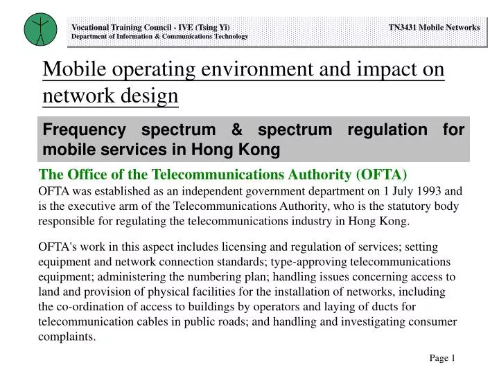
Mobile operating environment and impact on network design. Frequency spectrum & spectrum regulation for mobile services in Hong Kong. The Office of the Telecommunications Authority (OFTA)

E N D
Mobile operating environment and impact on network design Frequency spectrum & spectrum regulation for mobile services in Hong Kong The Office of the Telecommunications Authority (OFTA) OFTA was established as an independent government department on 1 July 1993 and is the executive arm of the Telecommunications Authority, who is the statutory body responsible for regulating the telecommunications industry in Hong Kong. OFTA's work in this aspect includes licensing and regulation of services; setting equipment and network connection standards; type-approving telecommunications equipment; administering the numbering plan; handling issues concerning access to land and provision of physical facilities for the installation of networks, including the co-ordination of access to buildings by operators and laying of ducts for telecommunication cables in public roads; and handling and investigating consumer complaints.
Radio Frequency Spectrum Assignment The aim is to ensure efficient utilization of the radio frequency spectrum. OFTA's responsibilities include the assignment of radio frequencies, investigation into interference complaints, licensing private telecommunications services, prosecution of illegal use of telecommunications equipment, and coordination with frequency management authorities outside Hong Kong to prevent interference between radio services. The table of frequency allocations publishing by OFTA in accordance with the Region 3 (Asia-Pacific Region) allocations under the Radio Regulations are applicable to Hong Kong, the allocations which have been adopted by Hong Kong, as well as the band plans in use in Hong Kong. The table of frequency allocations is intended to provide a reference for spectrum management, radiocommunication systems design, and other related areas of applications.
Radio Spectrum Advisory Committee • The terms of reference of the Radio Spectrum Advisory Committee are as follows - • To advise the Telecommunications Authority in the planning of the use of the radio frequency spectrum. • To advise the Telecommunications Authority in the formulation of the strategies, policies and procedures in the management of the radio frequency spectrum. • To advise the Telecommunications Authority in the formulation of Hong Kong's position at, and contributions to, international and regional forums on issues related to the management of the radio frequency spectrum.
Fading or multipath characteristics of a radio wave Since the antenna height of the mobile unit is lower than its typical surroundings, and the carrier frequency wavelength is much less than the sizes of the surrounding structures, multipath waves are generated. Radio waves arrive at a mobile receiver from different directions with different time delays or results from the motion of the scatterers of the radio waves (e.g., cars, trucks, vegetation). They combine via vector addition at the receiver antenna to give a resultant signal with a large or small amplitude. As a result, a receiver at one location may experience a signal strength several tens of dB different from a similar receiver located only a short distance away. It should also be noted that whenever relative motion exists there is a Doppler shift in the received signal. Multipath channel models, delay spread, path loss, doppler shift Figure.1 The multipath fading
At the mobile unit, the sum of the multipath waves causes a signal-fading phenomenon. The signal fluctuates in a range of about 40 dB (10 dB above and 30 dB below the average signal). The nulls of the fluctuation are roughly occurred at every half wavelength in space. If the mobile unit moves fast, the rate of fluctuation will be fast. Short-term Fading S(t) Long-term Fading L(t) Signal Strength dB Time (t) Figure.2 The fading characteristics of a mobile signal
The fading characteristics of a mobile radio signal is shown in the above figure. a. The rapid fluctuations caused by the local multipath are known as fast fading (Rayleigh fading). Fast fading is usually observed over distances of about half a wavelength. For VHF and UHF, a vehicle traveling at 30 miles per hour can pass through several fast fades in a second. b. The long-term variation in the mean level is known as slow fading (log-normalfading).The slow fading is caused by movement over distances large enough to produce gross variations in the overall path between the base station and the mobile. The mobile received signal R(t) can be expressed as: R(t) = L(t)S(t) Where L(t) = the long term fading S(t) = the short term fading
Fading Channel Models For short-term fading, there are two model of multipath channel models - Rayleigh fading and Rician fading Rayleigh fading is receiving a large number of reflected and scattered waves but no line of sight signal is received. Figure.3 The Rayleigh fading
Rician fading is receiving a set of reflected waves and a strong dominant or line of sight signal. Figure.4 The Rician fading
Multipath waves bounce back and forth due to the buildings and houses, they form many standing-wave pairs in space. Those standing-wave pairs are summed together and become an irregular wave-fading structure. When a mobile unit is standing still, its receiver only receives a signal strength at that spot, so a constant signal is observed. When the mobile unit is moving, the fading structure of the wave in the space is received. It is a multipath fading. The recorded fading becomes fast as the vehicle moves faster. Radio path Propagation loss Medium Figure.5 The Mobile radio environment
Under a multipath fading condition, the adverse effects will added on the digital cellular signal. 1.Rapid fluctuation of the signal amplitude and phase. 2.Dispersion or delay spread 3.Inter-Symbol interference 4.Different attenuation at different carriers and at different locations The frequency hopping of mobile service will also increases the quality of reception. In noise limited systems, frequency hopping helps to average out the effects of fast fading and is particularly useful at low signal levels. Frequency hopping provides interference diversity when hopping time slots. It is especially useful when the interleaving and channel coding capability is inadequate to deal with the channel errors.
System engineers are interested the fading in terms of level crossing rate and average fade duration below a specified level to select transmission bit rates, word lengths and coding schemes in digital radio systems. Both level crossing rate and average fade duration are the second-order statistics of fading. • Level crossing rate (lcr) • The average number of times per second that the signal envelope crosses a specified level R. • Where • r = the ratio between level R and the RMS amplitude of the fading envelope. Approximated expression
ii. Average Fade Duration is defined as Example 1. A cellular system of 900MHz, there is a vehicle receiver moving with speed of 24km/h. Calculate the level-crossing rate at a level of -10dB and average duration of fade. A typical ratio diagram is shown as follows Figure 2. A curve of N(R) against signal level
Initial Transmitted Pulse Base Station Antenna iii. Delay Spread The radio signal follows different paths which has a different travelling time. So an impulse is received at the receiver, it is no longer an impulse but rather a pulse that is spread and call the delay spread. The measured data indicate that the mean delay spreads are different in different kinds of environment. The situation is shown in the following figure. Received Pulses Figure 3. Delay spread situation
Delay spread limits the transmission rate. The performance is governed by bit error rate required and iv. Coherence bandwidth The coherence bandwidth is the defined bandwidth in which either the amplitudes or the phases of two received signals have a high degree of similarity. The delay spread is a natural phenomenon, and the coherence bandwidth is a defined creation related to the delay spread. A coherence bandwidth for two fading amplitudes and random phases of two received signals are Amplitude : Bc = __1__ Phase : B’c = __1__ 2 , 4 Where = the different between two received signal either in amplitude or phases
v. Path loss In general, the propagation path loss increases not only with frequency but also with distance. C R-2 = R-2 (free space) Where C = received carrier power R = distance measured from the transmitter to the receiver = constant The difference in power reception at two different distances R1 and R2 will result as C2 = R2-2C dB = C2 – C1 dB C1 R1 , = 20 log(R1/R2) In a real mobile radio environment, the propagation path loss slope varies as C R- = R- Usually lies between 2 and 5 depending on the actual conditions. Of course cannot be lower than 2, which is the free-space condition.
vi. Doppler shift For a vehicle moving with a constant velocity v, the received carrier is Doppler shifted by • Where fd = the Doppler shift • v = the receiver velocity • l = the carrier wavelength • = the horizontal projection angle • The waves arriving from ahead of the vehicle have a positive Doppler shift but those coming from behind will cause a negative shift.
Example 2 A vehicle traveling at 80.5kmph receives signals at carrier frequency of 880MHz. The Doppler shift will be Ans. (80.5 x 1000 /3600) x 880 x 106 / 3x 108 = 66Hz
Classification of Built-up Areas • The propagation of radio wave s in the built-up areas is strongly influenced by the • environment that is described as: • Urban areas are dominated by tall buildings, offices, and other commercial structures. • b. Suburban areas contain residential houses and parks. • c. Rural areas contain open farmland with farm buildings, wooded areas, and forests. Outdoor to Indoor and Pedestrian Radio Environment
In order to estimate the path loss at different environment, several models have been derived. In the following, there is a map which shows the power differences between that of radial and perpendicular streets Figure.4 Power differences of streets
Within 1 Km (microcell), the power received at perpendicular street has a drastically difference from that of radial street. It is more pronounced at a close-in location. • When the mobile unit is 1Km or further away from the base station (macrocell), there is no power difference between that of perpendicular and radial streets. The reason is that for the streets close to the base station, the buildings only cause a few reflected waves to reach the close-in corner. But for the far-out corner, the probability for reflected waves to reach is high. Thus, the far-out corner has similar power level as in the radial street. From the above phenomenon, we can see that the layout of the building blocks will greatly affect the signal propagation.
Lee marcocell Prediction model Lee marcocell received signal can be modelled by the following equations:
Where o is the adjustment factor is an attenuation factor (0<<1) due to the mobile radio environment Pr1 is the strength at one mile. (i.e. At a frequency 800MHz with 10W and 6dB antenna gain, the Pr1 is found to be -61.7dBm.) h1 is the height of the base-station antenna at 100ft ro is equals to 1km is the path loss slope
L() is the diffraction loss. The hp, r1 and r2 are defined in the following figure Figure 5. Effects of knife-edge obstructions on transmitted radio waves
An approximate solution of is shown in the following equations. The diffraction loss can be obtained from the graph of figure 6.
Lee's microcell model Figure 7. The propagation mechanics of low antenna height at the cell site When the size of a cell is small, less than 1km. The buildings directly affect the received signal strength level. The received signal at the mobile unit is coming from the multipath reflected waves, not from the waves penetrating through the buildings. It is found that the larger the number of the building blocks and the size of the blocks, the higher the signal attenuation. The estimation equation is
Where Pt is the ERP in dBm LB is the loss due to building blocks. (Typical value is -20dB when the block length is greater than 500ft.) Lloss(dA,h1) is the line of sight path loss at distance dA and antenna height h1.
To simplify the calculation, a parameter plot is shown in figure 8. From the graph, the line of sight loss and building block can be found directly. Figure 8. Microcell parameters
Example of a microcell path loss prediction a. Digitalize a building layout map
Identify the street blocks • Calculate the density of the ith street block (building area / street area) and label on the map • Take the line of sight path loss from curve a with antenna height adjustment • Calculate the total equivalent block length, such as • Lb = a x 0.347 + b x 0.31 + c x 0.41 • Find Lb from curve b. • f. The predicted signal strength is obtained by
In a real environment, the above calculation is just an estimation. The exact values will be affected by effect of • Street orientation • In urban areas, streets that run radically from the base station tend to enhance the received signal because of channeling effect. At frequencies of 1 GHz and lower, the effect is appreciably less. • Foliage • The presence of vegetation produces constant loss, independent of distance between communication terminals that are spaced 1km or more apart. A measured result is shown in the following figure
Frequency (MHz) Loss(dB) 150 40 300 14 1000 4 • Attenuation within tunnel • In the following, there are some data about the loss for different frequencies. • Nowaday, leaky-feeder (leaky-coaxial cable) techniques become increasingly important to provide adequate coverage and reduce interference in tunnel or in other confined space area Signal level Distance RF
Building and structures • Building Penetration losses is the main factor for analysis the coverage of in-door area from the out-door transmitters. • Mean Penetration Loss = Outdoor Signal – Indoor Signal • Signal inside building also assume to be in long-term fading