Download
1 / 38
380 likes | 497 Views
Flat clustering approaches for high-throughput omic datasets. Sushmita Roy BMI/CS 576 www.biostat.wisc.edu/bmi576 sroy@biostat.wisc.edu Nov 7 th , 2013. Key concepts to take away. What are high-throughput methods and datasets?

E N D
Flat clustering approaches for high-throughput omic datasets Sushmita Roy BMI/CS 576 www.biostat.wisc.edu/bmi576 sroy@biostat.wisc.edu Nov 7th, 2013
Key concepts to take away • What are high-throughput methods and datasets? • What are different computational approaches to analyze these datasets? • What does clustering let us do? • What are different clustering methods? • How do we evaluate the result of a clustering method?
Why omes and omics? • To understand how cells function • To understand what goes wrong with a system • To better predict risk of a disease • To develop personalized treatments In general, we want to understand cells as “systems”
Understand a cell as a system • Requires we identify the parts of a system • Requires we understand how these parts are put together • Clustering • Network inference • Network analysis • Predictive models
Understanding cells requires multiple types of measurements, model building and refinement Uwe Sauer, Matthias Heinemann, Nicola Zamboni, Science 2007
High-throughput datasets and “omes” • Aim to measure as many components of a cells simultaneously • Types of omes • Genome: collection of DNA in a cell • Transcriptome: all the RNA in cell • Proteome: all the proteins in a cell • Metabolome: all the metabolites present in a cell • Epigenome: all the chemical modifications on the genome • Interactome: all the interactions within a cell
Measuring transcriptomes mRNAs genes • What is varied: individuals, strains, cell types, environmental conditions, disease states, etc. • What is measured: RNA quantities for thousands of genes, exons or other transcribed sequences
Measuring gene expression • Microarrays • cDNA/spotted arrays • Affymetrix arrays • Sequencing • RNA-seq
Microarrays • A microarray is a solid support, on which pieces of DNA are arranged in a grid-like array • Each piece is called a probe • Measures RNA abundances by exploiting complementary hybridization • DNA from labeled sample is called target
cDNA Microarrays • RNA is isolated from matched samples of interest, and is typically converted to cDNA. It is labeled with fluorescent dyes, and then hybridized to the slide. Also look at this animation: http://www.bio.davidson.edu/courses/genomics/chip/chip.html
Microarray measurements • Can’t detect the absolute amount of mRNA present for a given gene, but can measure a relative quantity • For two color arrays, the measurements represent • Typically, we are working with log ratios: • More positive means high, • More negative means low • where red is the test expression level, and green is the reference level for gene G in the ithexperiment
Commonly asked questions from expression datasets • If we measure gene expression in a normal versus disease cell type, which genes have different expression levels across two groups? • Differential expression • Which genes seem to be changing together? • Clustering genes based on expression profiles of genes across all conditions • Which treatments/individuals have similar profiles? • Clustering samples based on gene expression profiles of all genes • What does a gene do? • What functional class does a given gene belong • What class is a sample from? • e.g., does this patient have ALL or AML • How will this sample react to a particular drug?
Gene-expression profiles for yeast cell cycle • Rows represent yeast genes • Columns represent time points as yeast goes through cell cycle • Color represents expression level relative to baseline (red=high, green=low, black=baseline) Spellman 1998
Microarray data for n conditions and m genes Conditions 1.2 1.4 ……… 0.8 -2.3 .. . . . Is a tall matrix of numbers with rows corresponding to genes and columns corresponding to conditions Genes Many analyses of omic datasets starts with clustering
Clustering of gene expression data • Task definition • Distance metric • Hierarchical clustering • Top-down and bottom up • Flat clustering • K-means • Model-based clustering • Gaussian mixture models
Distance measures • Central to all clustering algorithms is a measure of distance between objects being clustered • Clustering algorithms aim to group “similar” things together • Defining the right similarity or distance is an important factor in getting good clusters • Most algorithms will work with symmetric dissimilarities • Dissimilarities may not be distances
Different dissimilarity measures • Euclidean distance • Manhattan distance
K-means clustering • Uses Euclidean distance • Aims to minimize the within cluster scatter • Within cluster scatter defined as Number of objects in cluster k Mean of cluster k
K-means algorithm • Given: K, number of clusters, a set X={x1,.. xN} of data points, where xi are p-dimensional vectors • Initialize • Select initial cluster means • Repeat until convergence • Assign each xi to cluster C(i) such that • Re-estimate the mean of each cluster based on new members
K-means: updating the mean • To compute the mean of the cth cluster All objects in cluster c Number of objects in cluster c
K-means stopping criteria • Assignment of objects to clusters don’t change • One can also fix the max number of iterations • One can also see whether the optimization criterion changes by a small value
Gaussian mixture model based clustering • K-means is hard clustering • At each iteration, a datapoint is assigned to one and only one cluster • We can do soft clustering based on Gaussian mixture models • Each cluster is represented by a distribution (in our case a Gaussian) • We assume the data is generated by a mixture of the Gaussians
Gaussian mixture model-based clustering • Each cluster is represented by a multi-variate Gaussian Covariance matrix Univariate Gaussian Bi-variate Gaussian
Gaussian mixture model clustering • A model-based clustering approach • Enables us to have a generative model over the data as follows: • Roll a k-sided die to select one of the K Gaussians • Draw a sample from the selected Gaussian • The mixture model describes the probability of a data point x as
Learning a Gaussian mixture model • Again we assume we know how many Gaussians there are, that is we know what K is • We will assume that the co-variance matrix has zero off-diagonal elements. • For example for a 2-dimensional Gaussian we have: • So we need to estimate the means and variances
Learning a Gaussian mixture model (GMM) • We will use the expectation-maximization algorithm to learn GMM parameters • Assume we have N training data points (e.g. N genes) • Likelihood is
Using EM to learn the GMM • If we knew the cluster assignments estimating means and variances is easy • Take the data points in cluster c and estimate parameters for the Gaussian from clusterc • But we don’t. Instead we estimate the probability that a data point was generated by any of the K Gaussians • For each xi, let Zic denote whether xi is generated by Gaussianc • Zic is binary. • 1 if xi is generated by the cthGaussian • 0 if xi is not generated bycthGaussian
Expectation step • We would like to estimate the posterior probability of Zic=1 • cthGaussian generating data point xi • That is We will use to denote the posterior probability of the hidden variable
Maximization step • Here we need to estimate the parameters for each Gaussian • And the mixing weights Variance for the rth dimension
GMM clustering example Consider a one-dimensional clustering problem in which the data given are: x1 = -4 x2 = -3 x3 = -1 x4 = 3 x5 = 5 The initial mean of the first Gaussian is 0 and the initial mean of the second is 2. The Gaussians have fixed variance; their density function is: where denotes the mean of the Gaussian.
GMM clustering example • Here we have shown just one step of the EM procedure • We would continue the E- and M-steps until convergence
Demo details • 20 points generated from two Gaussians • We will estimate the mean, variance and the alpha for 10 iterations • Plot the likelihood.
Comparing k-means and GMMs • K-means • Hard clustering • Optimizes within cluster scatter • Requires estimation of means • GMMs • Soft clustering • Optimizes likelihood of data • Requires estimation of mean and covariance and mixture probabilities