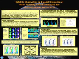
Satellite Observation and Model Simulation of Water Turbidity in the Chesapeake Bay

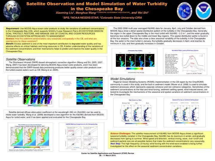
1. Satellite Observation and Model Simulation of Water Turbidity in the Chesapeake Bay Xiaoming Liu1, Menghua Wang 2 (PRINCIPAL GOVERNMENT INVESTIGATOR), and Wei Shi3 1SPS, 2NOAA/NESDIS/STAR, 3Colorado State University/CIRA The 2002-2008 multi-year averaged Kd(490) data for January, April, July and October derived from MODIS-Aqua show a detail spatial distribution pattern of the turbidity in the Chesapeake Bay. Generally, the region in the upper Chesapeake Bay is the most turbid with Kd(490) ~2-3 m-1, and the water gradually becomes less turbid down to the middle and lower Bay regions. This spatial distribution patter is found in all the four seasons. The data also show a clear seasonal variability of the turbidity in the Chesapeake Bay: the water is the most turbid in January, the turbidity gradually decreases in April, and reaches its minimum in July, and then gradually increases in October. Requirement: Use MODIS-Aqua ocean color products to study the variations of sediment concentrations in the Chesapeake Bay (CB), which supports NOAA’s 5-year Research Plan’s ECOSYSTEMS MISSION GOAL: PROTECT, RESTORE, AND MANAGE USE OF COASTAL AND OCEAN RESOURCES THROUGH ECOSYSTEM APPROACHES TO MANAGEMENT. Science:How the sediment concentrations vary seasonally and spatially in the CB, and what are mechanisms for these variations? Benefit:Excess sediment is one of the most important contributors to degraded water quality and has adverse effects on critical habitats and living resources in CB. A better understanding of the variations of the sediment concentrations and their mechanisms helps to predict and improve the water quality in the Chesapeake Bay. Normalized Water-Leaving Reflectance Spectra Chesapeake Bay Kd(490) January April July October The upper Chesapeake Bay region is also featured with enhanced water-leaving reflectance in the green and red bands between 555 and 645 nm. Reflecting the seasonal Kd(490) variation, highest reflectance at 645 nm occurs in the winter with value over 6% and the lowest during the summer with value less than 3%. a) b) c) d) January Satellite Observations The Shortwave Infrared (SWIR)-based atmospheric correction algorithm (Wang and Shi, 2005, 2007; Wang, 2007) has been developed for deriving MODIS-Aqua ocean color products, and it has been demonstrated that the SWIR-based data processing produces better quality ocean color products over the turbid coastal waters such as CB (Wang et al. 2009). April October July 0 1.5 3.0 m-1 2002-2008 Multi-Year Average Location of (39.29N, 76.32W) Model Simulations Regional Ocean Modeling Systems (ROMS) implementation in the CB region by the ChesROMS community is used in this study, and the built-in sediment model (Waner et al. 2008) is used to simulate sediment processes which represents separate cohesive and non-cohesive categories. Sensitivities of the sediment concentrations to the tidal and wind forcing, sediment settling speed, wind induced waves, are tested to investigate the mechanisms of the seasonal and spatial variations of sediment concentrations in the Chesapeake Bay. Comparisons of MODIS Ocean Color Products from NIR, SWIR, and NIR-SWIR Combined Methods Chlorophyll-a0.01-10 (mg/m3)(Log scale) Standard Data Processing July, 2005 Wang, M. and W. Shi (2007), “The NIR-SWIR combined atmospheric correction approach for MODIS ocean color data processing,” Optics Express, 15,15722-15733. Wang, M., S. Son, and W. Shi (2009), “Evaluation of MODIS SWIR and NIR-SWIR atmospheric correction algorithms using SeaBASS data,” Remote Sens. Environ., 113,635-644. Tidal Current vs. Wind Seasonal Forcing vs. Sediment Settling Speed Wind and Tide Tide Wind Winter, 0.01 mm/s Summer, 0.01 mm/s Summer, 0.1 mm/s NIR-SWIR Data Processing July, 2005 Satellite derived diffuse attenuation coefficient at the wavelength 490 nm (Kd(490)) can be used to relate water turbidity. Wang et al. (2009) developed a new algorithm for the Kd(490) derived from MODIS-Aqua for turbid water, and it has been applied and evaluated for the Chesapeake Bay. Kd(PAR) Matchup Comparisons for the Chesapeake Bay New Kd(490) for U.S. East Coastal Region NASA Standard Data Processing Science Challenges: The satellite measurement of Kd(490) from MODIS-Aqua shows a significant seasonal turbidity variation in the Chesapeake Bay. Kd(490) has its maximum in winter, and gradually decreases from spring to summer. Wind speed and direction, vertical mixing, wave, river runoff and sediment particle size are all possible factors that make the sediment concentrations vary seasonally. Next Step: The high-frequency (3-hourly) wind forcing with the wind-wave enabled is being further investigated for the effect on the seasonal sediment concentration variations. New Algorithm New Algorithm Wang, M., S. Son, and L. W. Harding Jr., “Retrieval of diffuse attenuation coefficient in the Chesapeake Bay and turbid ocean regions for satellite ocean color applications,” J. Geophys. Res. (2009).