Download
1 / 59
590 likes | 948 Views
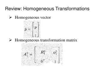
Homogeneous Transformations. CSE167: Computer Graphics Instructor: Steve Rotenberg UCSD, Fall 2006. Example: Distance Between Lines. We have two non-intersecting 3D lines in space

E N D
Homogeneous Transformations CSE167: Computer Graphics Instructor: Steve Rotenberg UCSD, Fall 2006
Example: Distance Between Lines • We have two non-intersecting 3D lines in space • Line 1 is defined by a point p1 on the line and a ray r1 in the direction of the line, and line 2 is defined by p2 and r2 • Find the closest distance between the two lines p2 r1 p1 r2
Example: Distance Between Lines • We want to find the length of the vector between the two points projected onto the axis perpendicular to the two lines p2 r1 p1 r2
Example: Distance Between Lines • Notice that the sign of the result might be positive or negative depending on the geometric configuration, so we should really take the absolute value if we want a positive distance • Also note that the equation could fail if |r1xr2|=0, implying that the lines are parallel. We should really test for this situation and use a different equation if the lines are parallel
Multiple Transformations • We can apply any sequence of transformations: • Because matrix algebra obeys the associative law, we can regroup this as: • This allows us to concatenate them into a single matrix: • Note: matrices do NOT obey the commutative law, so the order of multiplications is important
Multiple Rotations & Scales • We can combine a sequence of rotations and scales into a single matrix • For example, we can combine a y-rotation, followed by a z-rotation, then a non-uniform scale, and finally an x-rotation:
Multiple Translations • We can also take advantage of the associative property of vector addition to combine a sequence of translations • For example, a translation along vector t1 followed by a translation along t2 and finally t3 can be combined:
Combining Transformations • We see that we can combine a sequence of rotations and/or scales • We can also combine a sequence of translations • But what if we want to combine translations with rotations/scales?
Homogeneous Transformations • So we’ve basically taken the 3x3 rotation/scale matrix and the 3x1 translation vector from our original equation and combined them into a new 4x4 matrix (for today, we will always have [0 0 0 1] in the bottom row of the matrix) • We also replace our 3D position vector v with its 4D version [vx vy vz 1] (for today, we will always have a 1 in the fourth coordinate) • Using 4x4 transformation matrices allows us to combine rotations, translations, scales, shears, and reflections into a single matrix • In the next lecture, we will see how we can also use them for perspective and other viewing projections
Homogeneous Transformations • For example, a translation by vector r followed by a z-axis rotation can be represented as:
Arbitrary Axis Rotation • We can also rotate around an arbitrary unit axis a by an angle θ
Euler’s Theorem • Euler’s Theorem: Any two independent orthonormal coordinate frames can be related by a sequence of rotations (not more than three) about coordinate axes, where no two successive rotations may be about the same axis. • Not to be confused with Euler angles, Euler integration, Newton-Euler dynamics, inviscid Euler equations, Euler characteristic… • Leonard Euler (1707-1783)
Euler’s Theorem • There are two useful ways of looking at Euler’s theorem in relationship to orientations: • It tells us that we can represent any orientation as a rotation about three axes, for example x, then y, then z • It also tells us that any orientation can be represented as a single rotation about some axis by some angle
Orientation • The term orientation refers to an object’s angular configuration • It is essentially the rotational equivalent of ‘position’, unfortunately however, there is no equally simple representation • Euler’s Theorem tells us that we should not need more than 3 numbers to represent the orientation • There are several popular methods for representing an orientation. Some of these methods use 3 numbers, and other methods use more than 3…
Orientation • One method for storing an orientation is to simply store it as a sequence of rotations about principle axes, such as x, then y, then z. We refer to this as Euler angles. This is a compact method, as it uses exactly 3 numbers to store the orientation • Another option is to represent the orientation as a unit length axis and a scalar rotation angle, thus using 4 numbers in total. This is a conceptually straightforward method, but is of limited mathematical use, and so is not terribly common • A third option is to use a 3x3 matrix to represent orientation (or the upper 3x3 portion of a 4x4 matrix). This method uses 9 numbers, and so must contain some extra information (namely, the scaling and shearing info) • A fourth option is to use a quaternion, which is a special type of 4-dimensional vector. This is a popular and mathematically powerful method, but a little bit strange… These are covered in Math155B and CSE169 • No matter which method is used to store the orientation information, we usually need to turn it into a matrix in order to actually transform points or do other useful things
Scale Transformations • The uniform scaling matrix scales an entire object by scale factor s • The non-uniform scaling matrix scales independently along the x, y, and z axes
Volume Preserving Scale • We can see that a uniform scale by factor s will increase the volume of an object by s3, and a non-uniform scale will increase the volume by sxsysz • Occasionally, we want to do a volume preserving scale, which effectively stretches one axis, while squashing the other two • For example, a volume preserving scale along the x-axis by a factor of sx would scale the y and z axes by 1/sqrt(sx) • This way, the total volume change is
Volume Preserving Scale • A volume preserving scale along the x axis:
Shear Transformations • A shear transformation matrix looks something like this: • With pure shears, only one of the constants is non-zero • A shear can also be interpreted as a non-uniform scale along a rotated set of axes • Shears are sometimes used in computer graphics for simple deformations or cartoon-like effects
Translations • A 4x4 translation matrix that translates an object by the vector r is:
Pivot Points • The standard rotation matrices pivot the object about an axis through the origin • What if we want the pivot point to be somewhere else? • The following transformation performs a z-axis rotation pivoted around the point r
General 4x4 Matrix • All of the matrices we’ve see so far have [0 0 0 1] in the bottom row • The product formed by multiplying any two matrices of this form will also have [0 0 0 1] in the bottom row • We can say that this set of matrices forms a multiplicative group of 3D linear transformations • We can construct any matrix in this group by multiplying a sequence of basic rotations, translations, scales, and shears
General 4x4 Matrix • We will later see that we can change the bottom row to perform viewing projections, but for now, we will only consider the standard 3D transformations • We see that there are 12 different numbers in the upper 3x4 portion of the 4x4 matrix • There are also 12 degrees of freedom for an object undergoing a linear transformation in 3D space • 3 of those are represented by the three translational axes • 3 of them are for rotation in the 3 planes (xy, yz, xz) • 3 of them are scales along the 3 main axes • and the last 3 are shears in the 3 main planes (xy, yz, xz) • The 3 numbers for translation are easily decoded (dx, dy, dz) • The other 9 numbers, however, are encoded into the 9 numbers in the upper 3x3 portion of the matrix
Affine Transformations • All of the transformations we’ve seen so far are examples of affine transformations • If we have a pair of parallel lines and transform them with an affine transformation, they will remain parallel • Affine transformations are fast to compute and very useful throughout computer graphics
Object Space • The space that an object is defined in is called object space or local space • Usually, the object is located at or near the origin and is aligned with the xyz axes in some reasonable way • The units in this space can be whatever we choose (i.e., meters, etc.) • A 3D object would be stored on disk and in memory in this coordinate system • When we go to draw the object, we will want to transform it into a different space
World Space • We will define a new space called world space or global space • This space represents a 3D world or scene and may contain several objects placed in various locations • Every object in the world needs a matrix that transforms its vertices from its own object space into this world space • We will call this the object’s world matrix, or often, we will just call it the object’s matrix • For example, if we have 100 chairs in the room, we only need to store the object space data for the chair once, and we can use 100 different matrices to transform the chair model into 100 locations in the world
ABCD Vectors • We mentioned that the translation information is easily extracted directly from the matrix, while the rotation information is encoded into the upper 3x3 portion of the matrix • Is there a geometric way to understand these 9 numbers? • In fact there is! The 9 constants make up 3 vectors called a, b, and c. If we think of the matrix as a transformation from object space to world space, then the a vector is essentially the object’s x-axis rotated into world space, b is its y-axis in world space, and c is its z-axis in world space. d is of course the position in world space.
Orthonormality • If the a, b, and c vectors are all unit length and perpendicular to each other, we say that the matrix is orthonormal • Technically speaking, only the upper 3x3 portion is orthonormal, so the term is not strictly correct if there is a translation in the matrix • A better term for 4x4 matrices would be to call it rigid implying that it only rotates and translates the object, without any non-rigid scaling or shearing distortions
Orthonormality • If a 4x4 matrix represents a rigid transformation, then the upper 3x3 portion will be orthonormal
Example: Move to Right • We have a rigid object with matrix M. We want to move it 3 units to the object’s right
Example: Move to Right • We have a rigid object with matrix M. We want to move it 3 units to the object’s right M.d = M.d + 3*M.a
Example: Target ‘Lock On’ • For an airplane to get a missile locked on, the target must be within a 10 degree cone in front of the plane. If the plane’s matrix is M and the target position is t, find an expression that determines if the plane can get a lock on. • t M
Example: Target ‘Lock On’ • For an airplane to get a missile locked on, the target must be within a 10 degree cone in front of the plane. If the plane’s matrix is M and the target position is t, find an expression that determines if the plane can get a lock on. b • t d c a
Example: Target ‘Lock On’ • We want to check the angle between the heading vector (-c) and the vector from d to t: • We can speed that up by comparing the cosine instead ( cos(10°)=.985 )
Example: Target ‘Lock On’ • We can even speed that up further by removing the division and the square root in the magnitude computation: • All together, this requires 8 multiplications and 8 adds
Position Vector Dot Matrix y v=(.5,.5,0,1) x (0,0,0) Local Space
Position Vector Dot Matrix b Matrix M y y d a v=(.5,.5,0,1) x x (0,0,0) (0,0,0) Local Space World Space
Position Vector Dot Matrix b v’ y y d a v=(.5,.5,0,1) x x (0,0,0) (0,0,0) Local Space World Space
Position vs. Direction Vectors • Vectors representing a position in 3D space are expanded into 4D as: • Vectors representing direction are expanded as:
Matrix Dot Matrix • The abcd vectors of M’ are the abcd vectors of M transformed by matrix N • Notice that a, b, and c transform as direction vectors and d transforms as a position
Identity • Take one more look at the identity matrix • It’s a axis lines up with x, b lines up with y, and c lines up with z • Position d is at the origin • Therefore, it represents a transformation with no rotation or translation
Determinants • The determinant of a 4x4 matrix with no projection is equal to the determinant of the upper 3x3 portion
Determinants • The determinant is a scalar value that represents the volume change that the transformation will cause • An orthonormal matrix will have a determinant of 1, but non-orthonormal volume preserving matrices will have a determinant of 1 also • A flattened or degenerate matrix has a determinant of 0 • A matrix that has been mirrored will have a negative determinant
Inversion • If M transforms v into world space, then M-1 transforms v′ back into object space