Download

1 / 51
510 likes | 518 Views
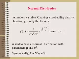
NORMAL DISTRIBUTION. Probability Distributions. In probability and statistics, a probability distribution is a mathematical description of a random phenomenon in a way that describes the probabilities of events happening. There are many forms this can take For example:

E N D
Probability Distributions In probability and statistics, a probability distribution is a mathematical description of a random phenomenon in a way that describes the probabilities of events happening. There are many forms this can take For example: For the random variable “the height of a randomly chosen 15 year old New Zealander” we could represent the probabilities of different heights as…. A table or a histogram Prob.
Statisticians are very keen to model a probability distribution. A common way to do this is to use a mathematical curve. This is similar to a parabola or a cubic, but the area under the entire curve is 1, signifying that the probability of all possible cases is 1 or 100%. Statisticians are keen because if they can find a good model estimate for the distribution, powerful statistical anlyses can quite readily be applied to it.
One of the more frequently used model used is the Normal distribution. We’re going to do a lot of work on this distribution, and your going to wonder, why all the fuss for this particular curve? Why are we so keen to see if it models my distribution well? Well, I assure you, if you follow through to higher studies in statistics, you will find that confirming that the data can be well approximated by a Normal distribution is huge, because the amount of tools available once this is confirmed increases substantially
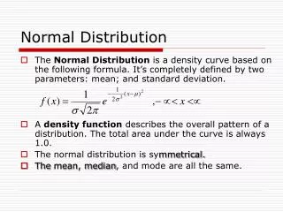
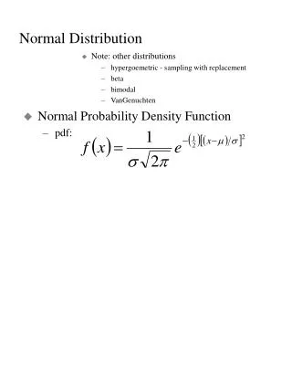
The Normal Distribution The normal distribution curve has a complicated formula: (You will not need to use this formula) Slightly more complicated then your Average quadratic! The shape of the curve depends on 2 parameters: (Mean) (standard deviation)
Normal Distribution • The mean (μ) is in the middle of the curve and changing the mean moves the curve right and left. • The standard deviation (σ) changes the steepness of the curve. A big standard deviation pulls the curve wide and a small standard deviation squeezes the curve narrow.
Some features • It is bell-shaped • It is symmetrical about the mean • It extends from -∞ to +∞ • The total area under the curve is 1
Approximately 95% of the distribution lies within two standard deviations from the mean.
Approximately 99.9% of the distribution lies within three standard deviations from the mean.
Regular Normal Question The area under the curve between any two -values is the probability of that event happening E.g. Weights of fish in a certain lake are found to be Normally Distributed with a mean of 5 kg and a standard deviation of 1.5 kg. Find the probability that a fish chosen at random will weigh between 5 and 6 kg. Probability of fish being between 5 and 6 kg 5 6
This can be done by your calculator. Go to Stat Dist Norm Ncd Make sure DATA is on ‘Var’ not ‘List’ Lower: the lower end of the shaded area (this is -9999999999 if there is no lower limit) Upper: the upper end of the shaded area (this is 9999999999 if there is no upper limit) REMEMBER: σ is the standard deviation and μ is the mean (I’ve seen way too many students mix this up on a test)
EXAMPLES Weights of fish in a certain lake are found to be Normally Distributed with a mean of 5 kg and a standard deviation of 1.5 kg. Find the probability that a fish chosen at random will weigh between 5 and 6 kg. Find the probability that a fish chosen at random will weigh less than 4 kg Find the probability that a fish chosen at random will weigh more than 7 kg The probability that a fish chosen at random will weigh between 3 and 8 kg The probability that a fish chosen at random is between 3 and 4 kg
Batteries for a transistor radio have a mean life under normal usage of 160 hours, with a standard deviation of 30 hours. Assuming a normal distribution: • Calculate the percentage of batteries which have a life between 150 hours and 180 hours. 37.8%
Batteries for a transistor radio have a mean life under normal usage of 160 hours, with a standard deviation of 30 hours. Assuming a normal distribution: • Calculate the range, symmetrical about the mean, within which 75% of the battery lives lie. 125.5, 194.5
This can be done by your calculator too Go to Stat Dist Norm Inv N Make sure DATA is on ‘Var’ not ‘List’ TAIL is the hard part to learn ‘Central’ means you want 2 -values such that the stated area is centrally located, with equal portions either side of the mean. ‘Left ‘means the area you are quoting is the shaded area under the curve going from that x-value off to the the left ‘Right’ means the area you are quoting is the shaded area under the curve going from that x-value off to the the right REMEMBER: σ is the standard deviation and μ is the mean (I’ve seen way too many students mix this up on a test)
EXAMPLES • Weights of fish in a certain lake are found to be Normally Distributed with a mean of 5 kg and a standard deviation of 1.5 kg. • Find the weight that 80% of fish weigh less than • Find the weight that 60% of fish weigh more than • The best tasting fish can be found in 30% of weights either side of the mean. Between which weights are the best tasting fish. • Reasonable tasting fish are above the bottom 10% but below the top 10%. Between which weights are the reasonable tasting fish? • A special breed called the CDA kingfish are heavier than the bottom 5% but can only reach their weights are within the bottom 20%. Between what weights are the CDA kingfish.
The heights of female students at a particular school are normally distributed with a mean of 169 cm and a standard deviation of 9 cm • Given that 80% of these female students have a height less than h cm, find the value of h. • Given that 60% of these female students have a height greater than s cm, find the value of s.
EXAMPLES The results of an entrance test are Normally distributed with a mean of 54 marks and a standard deviation of 12 marks. The top 5% get a full scholarship. The bottom 30% don’t get in. If the mark attained is between the mean and the next 30% of marks the students pay full fees. The marks higher than 80% of marks but less than 90% of marks are given partial scholarships. • What mark is required to get a full scholarship • Below what mark do you not get in. • What is the highest mark for which you will pay full fees. • What are the marks between which you get a partial scholarship.
IS USING A NORMAL DISTRIBUTION JUSTIFIED? As the good old saying goes: "All models are wrong, but some are better than others” Watch “Justifying use of Normal Distribution” video
As the good old saying goes: "All models are wrong, but some are better than others" • The Normal distribution is amazing, it ‘works’ for so many random processes we want to know something about, probably more than any theoretical distribution. • BUT, it is not an exact science. • Everything you have just been calculating is, essentially… wrong.
Let’s do a simple question…. When we are told that fish in a Lake are Normally distributed (with a mean of 5 and SD of 1.5)…and from that we calculate that the next fish I catch has 75% probability of weighing less than 6 kg… we’re wrong, it’s not going to actually be 75% ! You see, the Normal distribution is somewhat like a line of best fit, and hopefully the fit is so close to reality, that when you use it's curve, the probability found is only marginally off. So let's say the true probability of a fish weighing less than 6 kg is actually 77%, we can live with that, our answer was close. But if it were way off, there would be a problem. An excellence skill is FIRST deciding (with justification) whether the Normal distribution is a good enough estimate THEN go ahead and work out the probability, inverse question, etc.
So how does this (usually) look in year 12? Well, often when studying a random event, an experiment is carried out, and data collected. This data can often be represented as a histogram. A good way ofinformally assessing if a Normal distribution is a good fit for the random event we want to know something about, is to see if the histogram has features similar to a Normal Distribution This is a very regular question in the year 12 exam In order to do it, we need to first consider the things that make a Normal distribution a Normal distribution, what are some of it’s defining properties?
Properties: • SHAPE • The Normal distribution is symmetrical. There is is a line of symmetry at the mean. • The symmetry has a distinctive “bell-shape”. • The Normal Distribution is uni-modal • SPREAD • 95% of the Normal Distribution is within 2 standard deviation • . |two thirds is within 1.| |95 % is within 2 | | 99% is within 3 | • CENTRE • The mean=median=mode for the Normal distribution (as with any truly symmetrical distribution) (see next slide for how to estimate mean when data is not symmetrical) • The Normal distribution is a continuous distribution.
Extra For Experts: Calculating (Use My Calculator To Find) Mean And Standard Deviation From Histogram • MENU, STAT • Type in the X values into List 1 (in the case of a histogram use the middle of the bin as x-value) • Type the corresponding frequency into List 2 • Go to SET and set 1 X VAR X LIST: List 1 and 1 VAR FREQ: List 2 • CALC (F2) • 1 VAR (F1) • X with a bar on top approximates well the mean. • Sx approximates well the sample standard deviation
I will now use formal (university level) methods to check for normality.Which one do you think is better approximated by a Normal Distribution Very strong evidence that this data is not well modelled by a Normal Distribution. Another distribution should be considered Reasonable to assume the use of a Normal Distribution for modelling
Very strong evidence that this data is not well modelled by a Normal Distribution. Another distribution should be considered Reasonable to assume the use of a Normal Distribution for modelling At such a small sample size, it’s only natural that the shape of our variable is yet to settle. It is only logical at this sample size to have some discrepancy from the model At such a large sample size, even small discrepancies from the model are concerning
LESSON • For a small sample, we have to give leigh way, sometimes data which is well approximated by the Normal distribution doesn’t look so good because the sample is small. Remember, with a small sample we can give that leigh way. • With a bigger sample, we should be more stringent. In a bigger sample, the data should be approaching the true distribution, so…we cut it less slack
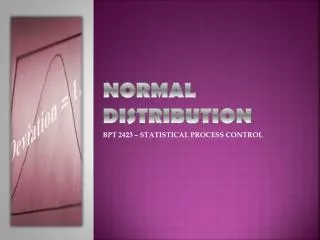
THE STANDARD NORMAL DISTRIBUTION • Has a mean of zero and a standard deviation of one.
Every single normal distribution ever can be standardized. I.E. Every normal distribution can be transformed (quite miraculously) to a ‘standard’ normal curve with mean 0 and standard deviation 1To represent this in a sketch, we center our normal curve on 0 (because that is the mean) and convert any x-value of interest into a ‘z-score’ using the formula: A z score always reflects the number of standard deviations above or below the mean a particular score is.
E.g. A test was found to have a mean of 50 and a standard deviation of 10. What is the probability of a student who sat the test getting less than 70 Prob density function of Norm(mean=50, std dev=10) Shaded area = P(X<70) IF Transforms to this (norm distribution with mean=0, std dev=1) All x-values are put through the formula
Eg. A test was found to have a mean of 50 and a standard deviation of 10. What is the probability of a student who sat the test getting less than 70 Shaded area remains the same -1 -2 0 1 2 magnified
Applying the formula will always produce a transformed distribution with: • a mean of 0 and a standard deviation of 1 • the shaded area under the transformed curve stays the same as the shaded area under the original ‘real-life’ curveThis proves very useful when looking for a parameter
Finding a parameter The times, X, to run a certain race are Normally distributed with μ = 12.36 minutes. If 65% of runners take less than 14.11 minutes, find the standard deviation of X. Watch Finding the Parameters Video
Finding a parameter The lengths of basketball shoes made by Chike are Normally distributed with a standard deviation of 4 cm. If 20% of shoes measure more than 35 cm, find the mean length of the basketball shoes. See “Normal Answers.pdf” for a walk through this question
The speeds of cars passing a certain point on a motorway can be taken to be normally distributed. Observations show that of cars passing the point, 95% are travelling at less than 85 kph and 10% are travelling at less than 55 kph. Find the average speed of the cars passing the point See “Normal Answers.pdf” for a walk through this question 68 kph
The speeds of cars passing a certain point on a motorway can be taken to be normally distributed. Observations show that of cars passing the point, 95% are travelling at less than 85 kph and 10% are travelling at less than 55 kph. Find the proportion of cars that travel at more than 70 kph. 0.4282
The masses of boxes of oranges are normally distributed such that 30% of them are greater than 4.00 kg and 20% are greater than 4.53 kg. Estimate the mean and standard deviation of the masses. See “Normal Answers.pdf” for a walk through this question 3.13, 1.67
SOME OLD SCHOOL TECHNICAL NOTATION (UNLIKELY TO NEED THIS) P(X < x) INSIDE THE BRACKETS: X [Big X] is the random variable, it’s what we’re ‘measuring’ (Eg. the lengths of crocodiles) x [little x] is the specified value of the random variable, it is a specific ‘measurement’ within all the possibilities afforded by X (if x=175 it refers to crocodile(s) 175 cm long) So in practice it looks like: P ( X< 190 ) P(X<190) : means : (what is the probability that ) (the lengths of Crocodiles)(is less than 190cm) P(170<X<190): means: what is the probability that the lengths of crocodiles is more than 170 but less than 190cm. P(X> 190) means what is the probability that the lengths of crocodiles is more than 190 cm
In inverse Normal problems the probability is given and you have to find the x value for that fulfills said probability E.g. “What length are 30% of crocodiles less than?” is written P(X < x) = 0.3 if read it says: P(X< x ) = 0.3 (The Probability that) (lengths)(is less than) (x) (is) (0.3) Remember, when we have a number we are looking for but don’t know what it is we use a variable. That is why x [little x] is left as a variable in inverse questions, that is what we look for (that’s the answer).
EXAMPLES USING TECHNICAL NOTATION • Weights of fish (X) in a certain lake are found to be Normally Distributed with a mean of 5 kg and a standard deviation of 1.5 kg. • P(X < x) = 0.8, find x Find the weight that 80% of fish weigh less than • P(X > 4) = ? What percentage of fish weigh more than 4 kg • P(2<X<7) = > What percentage of fish weigh between 2kg and 7 kg
Sometimes the normal distribution (a continuous distribution) is used to approximate situations that are really discrete. One of the common occurrences of this is when the occurs when data is measured to the nearest whole number. • The distribution takes on the shape of a normal distribution. In fact, the normal curve was instigated by De Moivre as an approximation to the Binomial.
The discrete data is represented by its limits. You have to ask what is the furthest limits of continuous measurement that would include the X I am looking for? E.g. 7 becomes the interval Because anything above 6.5 will round up to & anything under 7.5 will round down to 7 So because anything over 6.5 would be rounded up to 7, and everything above 7 had to be included anyway