Download
1 / 18
210 likes | 252 Views
GRID SYSTEMS. Size and Shape of the earth: Approximate sphere - about 20 km wider at equator than poles. Circumference = 40,000 km (25,000 miles).

E N D
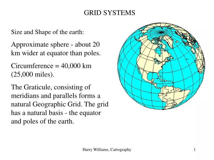
GRID SYSTEMS Size and Shape of the earth: Approximate sphere - about 20 km wider at equator than poles. Circumference = 40,000 km (25,000 miles). The Graticule, consisting of meridians and parallels forms a natural Geographic Grid. The grid has a natural basis - the equator and poles of the earth. Harry Williams, Cartography
Any point on the surface of the earth can be located in terms of its latitude and longitude (angles measured from the equator and Prime Meridian). Point P for example is at 30o north, 20o west. Latitude varies from 0o to 90o north or south. Longitude varies from from 0o to 180o east or west. Passes through Greenwich, England. Figure courtesy of Anthony P. Kirvan, and NCGIA Core Curriculum in GIScience. Harry Williams, Cartography
Degrees, Minutes, and Seconds • Angular measurement must be used to specify location on the earth's surface. A circle has 360 degrees, 60 minutes per degree, and 60 seconds per minute. Example: 45° 33' 22" (45 degrees, 33 minutes, 22 seconds). • At the equator 1 degree of longitude = 40,000 km/360 = 111 km. 1 minute = 111 km/60 = 1.85 km. 1 second = 1.85 km/60 = 30 m. Note: 1' latitude at the equator = 1 nautical mile; 1 knot = 1 nautical mile per hour. • Meridians converge, therefore at 60o latitude, 1 degree of longitude = 55.5 km. • There are 3,600 seconds per degree (60 x 60). • It is sometimes necessary to convert this conventional angular measurement into decimal degrees (e.g. often used in GIS’s). E.g. 45° 33' 22“ = 45° 2,002“ = 45° 2,002/3,600 = 45.55°. Harry Williams, Cartography
By convention, latitude is given before longitude. E.g. the corner of the map is: 33o 15’ N 97o 07’ 30” W Harry Williams, Cartography
Plane-coordinate Grid Systems. Problems with the Geographic Grid (Latitude and Longitude):1. Curved lines on many projections.2. Lines not equidistantly-spaced.3. Scale variations. A practical grid system should Have:1. Straight lines.2. Lines intersect at right angles.3. Lines equally-spaced.4. Grid squares have equal area. Two examples are: Universal Transverse Mercator Grid System State Plane Grid System Harry Williams, Cartography
Universal Transverse Mercator Grid System (UTM) A transverse cylindrical projection is used: A narrow strip, 6o of longitude wide, astride the central meridian has very little distortion. Harry Williams, Cartography
By moving the cylinder around the globe, 60 strips can be created: these are UTM grid zones, numbered 1-60. Harry Williams, Cartography
For example, grid zone 14 is centered on 99o west and runs through Texas. This zone covers 96o to 102o west. A 1-km grid is superimposed onto this map. The grid lines are numbered by their distance north from the equator and east from an imaginary base line which is arbitrarily located 500 km west of the central meridian (so the central meridian becomes the 500,000 m east grid line). Any point within the grid zone can be fixed by these two distances (a northing and an easting). Harry Williams, Cartography
The UTM reference: Zone 14: 621161 m E, 3349894 m N is a unique location within grid zone 14, accurate to the nearest meter. The grid zone number must be specified because this same reference occurs in all grid zones. When working on a map of a small area in the U.S. such as Denton, UTM grid references are usually given to the nearest hundred meters (i.e. the nearest 1/10 of a grid square; so 621161 m E would become 621200 m E). Also by convention, the zone number, the first digit in the easting, the first two digits in the northing and the two zeros (10’s and 1’s of meters) can be dropped. The example above would then become: 212499 …. This is a 6-digit UTM grid reference. Harry Williams, Cartography
For example, this point is 674100 m east and 3680300 m north in grid zone 14. It’s 6 digit UTM reference is: 741803 UTM grid tick Note: to find the original UTM reference, you can put the “missing’ numbers back, so 741803 becomes 674100 m east and 3680300 m north Harry Williams, Cartography
Plane-coordinate grid references like UTM references can be used to calculate distances between points because they are based on measured distances. For example, the UTM references 123456 and 333777 would have an easting separation of 33300 -12300 m = 21000 m = 21 km; and a northing separation of 77700 – 45600 m = 32100 m = 32.1 km. By Pythagoras theorem, the straight line distance between these points would be: sqrt 212 + 32.12 = sqrt 1471.41 = 38.36 km. 333777 38.36 km 32.1 km 21 km 123456 Harry Williams, Cartography
State Plane Grid System: In the United States, the State Plane System was developed in the 1930s and was based on the North American Datum 1927 (NAD27). This is similar to the UTM system. Older NAD-27 coordinates are in feet. Newer NAD-83 coordinates are usually in meters (can be in feet too). State plane systems were developed in order to provide local reference systems that were tied to a national datum (NAD-27, NAD-83). Larger states are divided into several zones. Lambert Conformal Conic projections are commonly used for rectangular zones with a larger east-west than north-south extent. Harry Williams, Cartography
Texas has 5 NAD-83 State Plane zones. Harry Williams, Cartography
Each zone has an origin with a false easting and northing to ensure positive coordinates. Harry Williams, Cartography
Some examples of State Plane Coordinates in Austin: Harry Williams, Cartography
State Plane coordinates are also shown on USGS maps (although there are only a few tick marks) Harry Williams, Cartography
Who uses the State Plane System? Many local governments do. North Central Texas Council of Governments (NCTCOG - www.dfwinfo.com) map data is usually in State Plane Coordinates. Example metadata is shown here for a map of city boundaries. Harry Williams, Cartography