Download
1 / 28
300 likes | 504 Views
Hypothesis Testing and Sample Size Calculation. Po Chyou, Ph. D. Director, BBC. Population mean(s) Population median(s) Population proportion(s) Population variance(s) Population correlation(s) Association based on contingency table(s). Coefficients based on regression model Odds ratio

E N D
Hypothesis TestingandSample Size Calculation Po Chyou, Ph. D. Director, BBC
Population mean(s) Population median(s) Population proportion(s) Population variance(s) Population correlation(s) Association based on contingency table(s) Coefficients based on regression model Odds ratio Relative risk Trend analysis Survival distribution(s) / curve(s) Goodness of fit Hypothesis Testingon
Hypothesis Testing 1. Definition of a Hypothesis An assumption made for the sake of argument 2. Establishing Hypothesis Null hypothesis - H0 Alternative hypothesis - Ha 3. Testing Hypotheses Is H0true or not?
Hypothesis Testing 4.Type I and Type II Errors Type I error: we reject H0but H0is true α= Pr(reject H0 / H0 is true) = Pr(Type I error) = Level of significance in hypothesis testing Type II error: we accept H0but H0is false = Pr(accept H0 / H0 is false) = Pr(Type II error)
Hypothesis Testing 5. Steps of Hypothesis Testing - Step 1 Formulate the null hypothesis H0 in statistical terms - Step 2 Formulate the alternative hypothesis Ha in statistical terms - Step 3 Set the level of significance αand the sample size n - Step 4 Select the appropriate statistic and the rejection region R - Step 5 Collect the data and calculate the statistic
Hypothesis Testing 5. Steps of Hypothesis Testing (continued) - Step 6 If the calculated statistic falls in the rejection region R, reject H0 in favor of Ha; if the calculated statistic falls outside R, do not reject H0
Hypothesis Testing 6. An Example A random sample of 400 persons included 240 smokers and 160 non-smokers. Of the smokers, 192 had CHD, while only 32 non-smokers had CHD. Could a health insurance company claim the proportion of smokers having CHD differs from the proportion of non-smokers having CHD?
Hypothesis TestingExample (continued) Let P1 = the true proportion of smokers having CHD P2= the true proportion of non-smokers having CHD - Step 1 H0 : P1 =P2 - Step 2 Ha : P1 P2 - Step 3 α = .05, n = 400
Hypothesis TestingExample (continued) - Step 4 statistic = = P1 - P2 where P1 = x1 ,P2 = x2 and P= x1 + x2 n1 n2n1 + n2 P(1-P) (1/n1 + 1/n2)
Hypothesis TestingExample (continued) - Step 5 P1= x1 = 192 = .80 240 n1 P2= x2 n2 = 32 = .20 160 P= x1 + x2 n1 + n2 = 192 + 32 = 224 = 0.56 240 + 160 400 =P1 - P2 = .80 - .20 = .60 = 11.84 > 1.96 P(1-P) (1/n1 + 1/n2) (.56) (1-.56) (1/240 + 1/160) .05066
Hypothesis TestingExample (continued) - Step 6 Reject H0 and conclude that smokers had significantly higher proportion of CHD than that of non-smokers. [P-value < .0000001]
Hypothesis Testing 7. Contingency Table Analysis The Chi-square distribution (2)
Hypothesis Testing Equation for chi-square for a contingency table 2 = (Oij - Eij )2 i, j Eij For i = 1, 2 and j =1, 2 2= (O11 - E11)2 + (O12 - E12)2 + (O21 - E21)2 + (O22 - E22)2 E11 E12E21 E22
Hypothesis Testing Equation for chi-square for a contingency table (cont.) E11= n1m1 E12= n1 - n1m1 = n1m2 n n n E21= n2m1 E22= n2 - n2m1 = n2m2 n n n
Hypothesis TestingExample : Same as before - Step 1 H0 : there is no association between smoker status and CHD - Step 2 Ha : there is an association between smoker status and CHD - Step 3 = .05, n = 400 - Step 4 statistic = 2= (O11 - E11)2 + (O12 - E12)2 + (O21 - E21)2 + (O22 - E22)2 E11 E12 E21 E22
Hypothesis TestingExample (continued) : Same as before - Step 5
Hypothesis TestingExample (continued) : Same as before E11= n1m1 = 240 * 224 = 134.4 n 400 E12= n1 -n1m1 = 240 - 134.4 = 105.6 n E21= n2m1 = 160 * 224 = 89.6 n 400 E22= n2 -n2m1 = 160 - 89.6 = 70.4 n - Step 5 (continued) Expectation Counts
Hypothesis TestingExample (continued) : Same as before - Step 5 (continued) 2= (O11 - E11)2 + (O12 - E12)2 + (O21 - E21)2 + (O22 - E22)2 E11E12E21 E22 = (192 - 134.4)2 + (48 - 105.6)2 + (32 - 89.6)2 + (128 - 70.4)2 134.4 105.6 89.6 70.4 = 24.68 + 31.42 + 37.03 + 47.13 = 140.26 > 3.841
Hypothesis TestingExample (continued) : Same as before - Step 6 Reject H0 and conclude that there is an association between smoker status and CHD. [P-value < .0000001]
Sample Size Estimation andStatistical Power Calculation Definition of Power Recall : = Pr (accept H0 / H0 is false) = Pr (Type II error) Power = 1 - = Pr(reject H0 / H0 is false)
Sample Size Estimationfor Intervention on Tick Bites Among Campers 1. Given that the proportion (PCON) of tick bites among campers in the control group is constant. 2. Given that the proportion (PINT) of tick bites among campers in the intervention group is reduced by 50% compared to that of the control group after intervention has been implemented. 3. Given that a one- or two- tailed test is of interest with 80% power and a type-I error of 5%. Assumptions
Sample Size Estimationfor Intervention on Tick Bites Among Campers Summary Table 1
Statistical Power Calculationfor Intervention on Obesity of Women in MESA 1. Given that the proportion (PCON) of women who are obese at baseline (i.e., the control group) is constant. There are a total of 840 women in the control group. Based on our preliminary data analysis results, approximately 50% of these 840 women at baseline are obese (BMI >= 27.3). 2. Given that the proportion (PINT) of women who are obese in the intervention group is reduced by 5% or more compared to that of the control group after intervention has been implemented. There are a total of 680 women who had been newly recruited. Based on our preliminary data analysis results, 50% of these 680 newly recruited women are obese. Assume that 60% of these women will agree to participate, we will have 200 women to be targeted for intervention. Assumptions
Statistical Power Calculationfor Intervention on Obesity of Women in MESA (continued) 3. Given that a one-tailed test is of interest with a type-I error of 5%, then the estimated statistical powers are shown in Table 1 for detecting a difference of 5% or more in the proportion of obesity between the control group and the intervention group. Assumptions Table 1
Reference “Statistical Power Analysis for the Behavioral Sciences” Jacob Cohen Academic Press, 1977
Take Home Message: • You’ve got questions : Data ? STATISTICS?... • Contact Biostatistics and consult with an experienced biostatistician • Po Chyou, Director, Senior Biostatistician (ext. 9-4776) • Dixie Schroeder, Secretary (ext. 1-7266) OR • Do it at your own risk