Download
1 / 19
190 likes | 266 Views
Learn about visual interpretation of first-order equations through slope fields and numerical approximations using Euler’s Method. Use Isoclines to sketch integral curves satisfying different initial conditions. Understand graphical insights on asymptotic behavior and Uniqueness Principle in differential equations.

E N D
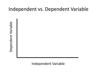
In the previous two sections, we focused on finding solutions to differential equations. However, most differential equations cannot be solved explicitly. Fortunately, there are techniques for analyzing the solutions that do not rely on explicit formulas. In this section, we discuss the method of slope fields, which provides us with a good visual understanding of first-order equations. We also discuss Euler’s Method for finding numerical approximations to solutions. We use t as the independent variable and write for dy/dt. The notation often used for time derivatives in physics and engineering, was introduced by Isaac Newton. A first-order differential equation can then be written in the form where F (t, y) is a function of t and y. For example, dy/dt = -tybecomes
It is useful to think of this equation as a set of instructions that “tells a solution” which direction to go. Thus, a solution passing through a point (t, y) is “instructed” to continue in the direction of slope F (t, y). To visualize this set of instructions, we draw a slope field, which is an array of small segments of slope F (t, y) at points (t, y) lying on a rectangular grid in the plane. To illustrate, let’s return to the differential equation In this case, F (t, y) = −ty. According to Example 2 of Section 9.1, the general solution is
To sketch the slope field for , we draw small segments of slope −ty at an array of points (t, y) in the plane. The slope field allows us to visualize all of the solutions at a glance. Starting at any point, we can sketch a solution by drawing a curve that runs tangent to the slope segments at each point. The graph of a solution is also called an integral curve.
Using IsoclinesDraw the slope field for and sketch the integral curves satisfying the initial conditions (a)y (0) = 1 and (b)y (1) = −2. Choose several values c and identify the curve F (t, y) = c, called the isocline of slope c. The isocline is the curve consisting of all points where the slope field has slope c. F (t, y) = y − t, so the isocline of fixed slope c has equation y − t = c, or y = t + c, which is a line. Consider the following values: • c= 0: This isocline is y= t. We draw segments of slope c= 0 at points along the line y = t. • c= 1: This isocline is y= t + 1. We draw segments of slope 1 at points along y = t + 1. • c= 2: This isocline is y= t + 2. We draw segments of slope 2 at points along y = t + 2. • c= −1: This isocline is y= t − 1. Slope Field
To sketch the solution satisfying y (0) = 1, begin at the point (t0, y0) = (0, 1) and draw the integral curve that follows the directions indicated by the slope field. Similarly, the graph of the solution satisfying y (1) = −2 is the integral curve obtained by starting at (t0, y0) = (1, −2) and moving along the slope field. Our last graph, shows several other solutions (integral curves). c Isoclines
GRAPHICAL INSIGHT Slope fields often let us see the asymptotic behavior of solutions (as t → ∞) at a glance. Figure 3(E) suggests that the asymptotic behavior depends on the initial value (the y-intercept): If y (0) > 1, then y (t) tends to ∞, and if y (0) < 1, then y (t) tends to −∞. We can check this using the general solution y (t) = 1 + t + Cet, where y(0) = 1 + C. If y (0) > 1, then C > 0 and y (t) tends to ∞, but if y (0) < 1, then C < 0 and y (t) tends to −∞. The solution y = 1 + t with initial condition y (0) = 1 is the straight line shown in Figure 3(D).
Newton’s Law of Cooling Revisited The temperature y (t) (°C) of an object placed in a refrigerator satisfies (t in minutes). Draw the slope field and describe the behavior of the solutions. Solution The function F (t, y) = −0.5(y − 4) depends only on y, so slopes of the segments in the slope field do not vary in the t-direction.
CONCEPTUAL INSIGHT Most first-order equations arising in applications have a uniqueness property: There is precisely one solution y(t) satisfying a given initial condition y (t0) = y0. Graphically, this means that precisely one integral curve (solution) passes through the point (t0, y0). Thus, when uniqueness holds, distinct integral curves never cross or overlap. Figure 5 shows the slope field of , where uniqueness fails. We can prove that once an integral curve touches the t-axis, it either remains on the t-axis or continues along the t-axis for a period of time before moving below the t-axis. Therefore, infinitely many integral curves pass through each point on the t-axis. However, the slope field does not show this clearly. This highlights again the need to analyze solutions rather than rely on visual impressions alone.
Euler’s Method produces numerical approximations to the solution of a first-order initial value problem: We begin by choosing a small number h, called the time step, and consider the sequence of times spaced at intervals of size h: c c c c In general, tk = t0 + kh. Euler’s Method consists of computing a sequence of values y1, y2, y3,…, yn successively using the formula c c c c Starting with the initial value y0 = y (t0), we compute y1= y0 + hF(t0, y0) , etc. The value yk is the Euler approximation to y(tk). We connect the pointsPk = (tk, yk) by segments to obtain an approximation to the graph of y (t).
GRAPHICAL INSIGHT The values yk are defined so that the segment joining Pk−1 to Pk has slope c c c c c c c c Thus, in Euler’s method we move from Pk−1 to Pk by traveling in the direction specified by the slope field at Pk−1 for a time interval of length h.
Use Euler’s Method with time step h = 0.2 and n = 4 steps to approximate the solution of c Our initial value at t0 = 0 is y0 = 3. Since h = 0.2, the time values are t1 = 0.2,t2 = 0.4,t3 = 0.6, and t4 = 0.8. We use F(t, y) = y − t2 to calculate c c c c c c c c c c c c c c c c c c c c c c c c c c c c c c c c
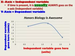
The figure shows the exact solution y (t) = 2 + 2t + t2 + et together with a plot of the points (tk, yk) for k = 0, 1, 2, 3, 4 connected by line segments.
CONCEPTUAL INSIGHT The time step h = 0.1 gives a better approximation than h = 0.2. In general, the smaller the time step, the better the approximation. In fact, if we start at a point (a, y (a)) and use Euler’s Method to approximate (b, y (b)) using N steps with h= (b − a)/N, then the error is roughly proportional to 1/N (provided that F(t, y) is a well-behaved function). This is similar to the error size in the Nth left- and right-endpoint approximations to an integral. What this means, however, is that Euler’s Method is quite inefficient; to cut the error in half, it is necessary to double the number of steps, and to achieve n-digit accuracy requires roughly 10n steps. Fortunately, there are several methods that improve on Euler’s Method in much the same way as the Midpoint Rule and Simpson’s Rule improve on the endpoint approximations (see Exercises 22–27).
Let y (t) be the solution of (a) Use Euler’s Method with time step h = 0.1 to approximate y (0.5). (b)We will not be using a CAS! (a) When h = 0.1, yk is an approximation to y (0 + k (0.1)) = y (0.1k), so y5 is an approximation to y (0.5). It is convenient to organize calculations in the following table. Note that the value yk+1 computed in the last column of each line is used in the next line to continue the process. c c c c c c c c c c c c c c c c c c c c c c c c c c c c c c c c c c Thus, Euler’s Method yields the approximation y (0.5) ≈ y5 ≈ 0.1.
![The Impact of [independent variable] On [dependent variable] Controlling for [control variable]](https://cdn0.slideserve.com/430545/the-impact-of-independent-variable-on-dependent-variable-controlling-for-control-variable-dt.jpg)