Download
1 / 101
1.16k likes | 1.45k Views
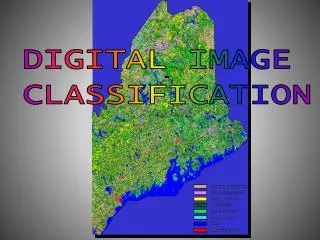
Image Classification. Chapter 12. Intro. Digital image classification is assigning pixels to classes (categories) Each pixel has as many digital values as there are bands Compare the values to pixels of known composition and assign them accordingly Each class (in theory) is homogenous.

E N D
Image Classification Chapter 12
Intro • Digital image classification is assigning pixels to classes (categories) • Each pixel has as many digital values as there are bands • Compare the values to pixels of known composition and assign them accordingly • Each class (in theory) is homogenous
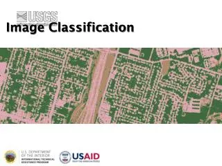
Intro • Direct uses • Produce a map of land-use/land-cover • Indirect use • Classification is an intermediate step, and may form only one of several data layers in a GIS • Water map vs water quality GIS
Intro • Classifier is a computer program that does some sort of image classification • Many different types available • No one method is “best” • Simplest is a point or spectral classifier • Considers each pixel individually • Simple and economic • Can’t describe relation to neighboring pixels
Intro • Spatial neighborhood classifiers consider groups of pixels • More difficult to program and more expensive
Intro • Supervised vs Unsupervised classification • Supervised requires the analyst to identify known areas • Unsupervised determines a set number of categories based on a computer algorithm • Hybrid classifiers are a mix of the two
Unsupervised classification • No previous knowledge assumed about data. • Tries to spectrally separate the pixels. • User has controls over: • Number of classes • Number of iterations • Convergence thresholds • Two main algorithms: Isodata and k-means
Informational Classes • Informational classes are categories of interest to the users • Geological units • Forest types • Land use
Spectral classes • Spectral classes are pixels that are of uniform brightness in each of their several channels • The idea is to link spectral classes to informational classes • However, there is usually variability that causes confusion • A forest can have trees of varying age, health, species composition, density, etc.
Classes • Informational classes then are usually composed of numerous spectral subclasses. • These subclasses may be displayed as a single unit on the final product • We often will want to examine how different the pixels within a class are • Look at variance and standard deviation
Variance • The Variance is defined as: • The average of the squared differences from the Mean. • Which is the square of the standard deviation, ie: σ2
The heights (at the shoulders) are: 600mm, 470mm, 170mm, 430mm and 300mm.
Now, we calculate each dogs difference from the Mean: To calculate the Variance, take each difference, square it, and then average the result: So, the Variance is 21,704.
And the Standard Deviation is just the square root of Variance, so: Standard Deviation: σ = √21,704 = 147 So, using the Standard Deviation we have a "standard" way of knowing what is normal, and what is extra large or extra small. Rottweillers are tall dogs. And Dachsunds are a bit short ... but don't tell them!
Differences between means • A crude estimate of might be to simply look at the differences in means between two classes • This is too simplistic since it does not account for differences in variability between the two • A better way is to look at normalized differences
NDWI • The Normalized Difference Water Index (NDWI) (Gao, 1996) • The SWIR reflectance reflects changes in both the vegetation water content and the spongy mesophyll structure in vegetation canopies, • The NIR reflectance is affected by leaf internal structure and leaf dry matter content but not by water content. • The combination of the NIR with the SWIR removes variations induced by leaf internal structure and leaf dry matter content, improving the accuracy in retrieving the vegetation water content (Ceccato et al. 2001).
Normalized Difference Snow Index (NDSI ) • Normalized Difference Vegetation Index • Normalized Difference Cloud Index (NDCI) is defined as a ratio between the difference and the sum of two zenith radiances measured for two narrow spectral bands in the visible and near-IR regions. • It provides extra tools to remove the radiative effects of the 3D cloud structure.
Unsupervised Classification • RS images are usually composed of several relatively uniform spectral classes • Unsupervised classification is the identification, labeling and mapping of such classes
Unsupervised Classification • Advantages • Requires no prior knowledge of the region • Human error is minimized • Unique classes are recognized as distinct units • Disadvantages • Classes do not necessarily match informational categories of interest • Limited control of classes and identities • Spectral properties of classes can change with time
Unsupervised Classification • Distance Measures are used to group or cluster brightness values together • Euclidean distance between points in space is a common way to calculate closeness • Euclidean metric is the "ordinary" distance between two points that one would measure with a ruler, and is given by the Pythagorean formula.
Euclidean Distance • Distance
Euclidean Distance • Example, the (Euclidean) distance between points (2, -1) and (-2, 2) • dist((2, -1), (2, 2)) • = √(2 - (-2))² + ((-1) - 2)² • = √(2 + 2)² + (-1 - 2)² • = √(4)² + (-3)² • = √16 + 9 • = √25 • = √5.
This can be extended to multiple dimensions (bands) Add the differences together Σ (dif)2 = 1,637 √1637 = 40.5 Euclidean Distance
Distances • There are a number of other distances that can be calculated • L1 distance is the sum of absolute differences between different bands • e.g. 8=12+30+23 = 73 for previous example
Example Landsat bands Near-IR band Red band
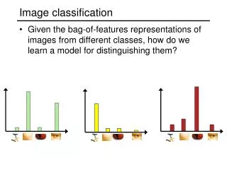
Example spectral plot • Two bands of data. • Each pixel marks a location in this 2d spectral space • Our eye’s can split the data into clusters. • Some points do not fit clusters.
K-means (unsupervised) • A set number of cluster centers are positioned randomly through the spectral space. • Pixels are assigned to their nearest cluster. • The mean location is re-calculated for each cluster. • Repeat 2 and 3 until movement of cluster centres is below threshold. • Assign class types to spectral clusters.
Example k-means 1. First iteration. The cluster centers are set at random. Pixels will be assigned to the nearest center. 2. Second iteration. The centers move to the mean-center of all pixels in this cluster. 3. N-th iteration. The centers have stabilized.
Key Components • Regardless of the unsupervised algorithm need to pay attention to methods for • Measuring distance • Identifying class centroids • Testing distinctness of classes
Decision Boundary • All classification programs try to determine classes based on “decision boundaries” • That is, divide feature space into an exhaustive set of nonoverlapping regions • Begin with a set of prelabeled points for each class (training samples) • Minimum Distance to Means – determine locus of points equidistant from class mean • Nearest neighbor – determine locus of points equidistant from the nearest member of 2 classes
Decision boundary Decision boundary
Decision Boundaries • Classification usually not so easy • Desired classes have distributions in feature space that are not obviously separated • Nearly always have to use more than three features (dimensions) • Wind up having to use discriminant functions
Supervised classification • Start with knowledge of class types. • Classes are chosen at start • Training samples are created for each class • Ground truth used to verify the training samples. • Quite a few algorithms. Here we will look at: • Parallelepiped • Maximum likelihood
Supervised Classification • Advantages • Analyst has control over the selected classes tailored to the purpose • Has specific classes of known identity • Does not have to match spectral categories on the final map with informational categories of interest • Can detect serious errors in classification if training areas are missclassified
Supervised Classification • Disadvantages • Analyst imposes a classification (may not be natural) • Training data are usually tied to informational categories and not spectral properties • Remember diversity • Training data selected may not be representative • Selection of training data may be time consuming and expensive • May not be able to recognize special or unique categories because they are not known or small
Supervised Classification • Training data • Specify corner points of selected areas • Assume that the correct ID is known • Often requires ancillary data (maps, photos, etc.) • Field work often needed to verify
Supervised Classification • Key Characteristics of Training areas • Number of pixels • Have several training areas for one category • A total of at least 100 pixels per category • Number depends on the number of categories, their diversity, and resources available • More areas also allow discarding ones that have too high a variance • Shape –not important, usually rectangular for ease
Supervised Classification • More Key Characteristics • Locations must be spread around the image and be easily transferred from map to image • Size must be large enough to estimate spectral characteristics and variations • Varies with sensor type and resolution • Varies with heterogeneity of area • Uniformity means that each training set should be as homogenous as possible
Idealized Sequence • Assemble information • Conduct field studies • Conduct preliminary study of scene to determine landmarks and assess image quality • Identify training areas • Evaluate training data • Edit training data if necessary
Feature Selection • Graphic Method – one of the first simple feature selection aids • Plot ±1σ in a bar graph
Feature Selection • Cospectral parallelepiped plots (ellipse plots) visual representation of separability in two dimensional feature space • Use mean and SD of training class statistics for each class, c, and band, k • Parallelepipeds represent mean ±1σ of each band for each class