Download
1 / 28
280 likes | 712 Views
Image classification by sparse coding. Feature learning problem. Given a 14x14 image patch x, can represent it using 196 real numbers. Problem: Can we find a learn a better representation for this? . Unsupervised feature learning.

E N D
Image classification by sparse coding
Feature learning problem • Given a 14x14 image patch x, can represent it using 196 real numbers. • Problem: Can we find a learn a better representation for this?
Unsupervised feature learning Given a set of images, learn a better way to represent image than pixels.
First stage of visual processing in brain: V1 The first stage of visual processing in the brain (V1) does “edge detection.” Green: Responds to white dot. Red: Responds to black dot. Actual simple cell Schematic of simple cell Also used in image compression and denoising. “Gabor functions.” [Images from DeAngelis, Ohzawa & Freeman, 1995]
Learning an image representation Sparse coding (Olshausen & Field,1996) Input: Images x(1), x(2), …, x(m)(each in Rn x n) Learn: Dictionary of bases f1, f2, …, fk (also Rn x n), so that each input x can be approximately decomposed as: s.t. aj’s are mostly zero (“sparse”) Use to represent 14x14 image patch succinctly, as [a7=0.8, a36=0.3, a41 = 0.5]. I.e., this indicates which “basic edges” make up the image. [NIPS 2006, 2007]
Sparse coding illustration Natural Images Learned bases (f1 , …, f64): “Edges” » 0.8 * + 0.3 * + 0.5 * Test example x»0.8 * f36+ 0.3 * f42+ 0.5 * f63 [0, 0, …, 0,0.8, 0, …, 0, 0.3, 0, …, 0, 0.5, …] = [a1, …, a64] (feature representation) Compact & easily interpretable
»0.6 * + 0.8 * + 0.4 * 15 28 37 »1.3 * + 0.9 * + 0.3 * 5 18 29 More examples Represent as: [0, 0, …, 0,0.6, 0, …, 0, 0.8, 0, …, 0, 0.4, …] Represent as: [0, 0, …, 0,1.3, 0, …, 0, 0.9, 0, …, 0, 0.3, …] • Method hypothesizes that edge-like patches are the most “basic” elements of a scene, and represents an image in terms of the edges that appear in it. • Use to obtain a more compact, higher-level representation of the scene than pixels.
Digression: Sparse coding applied to audio [Evan Smith & Mike Lewicki, 2006]
Digression: Sparse coding applied to audio [Evan Smith & Mike Lewicki, 2006]
Sparse coding details Input: Images x(1), x(2), …, x(m)(each in Rn x n) L1 sparsity term (causes most s to be 0) Alternating minimization: Alternately minimize with respect to fi‘s (easy) and a’s (harder).
Solving for bases Early versions of sparse coding were used to learn about this many bases: 32 learned bases How to scale this algorithm up?
Sparse coding details Input: Images x(1), x(2), …, x(m)(each in Rn x n) L1 sparsity term Alternating minimization: Alternately minimize with respect to fi‘s (easy) and a’s (harder).
Feature sign search (solve for ai’s) • Goal: Minimize objective with respect to ai’s. • Simplified example: • Suppose I tell you: • Problem simplifies to: • This is a quadratic function of the ai’s. Can be solved efficiently in closed form. • Algorithm: • Repeatedly guess sign (+, - or 0) of each of the ai’s. • Solve for ai’s in closed form. Refine guess for signs.
The feature-sign search algorithm: Visualization Current guess: Starting from zero (default)
The feature-sign search algorithm: Visualization Current guess: 1: Activate a2 with “+” sign Active set ={a2} Starting from zero (default)
The feature-sign search algorithm: Visualization Current guess: 1: Activate a2 with “+” sign Active set ={a2} Starting from zero (default)
The feature-sign search algorithm: Visualization Current guess: 2: Update a2 (closed form) 1: Activate a2 with “+” sign Active set ={a2} Starting from zero (default)
The feature-sign search algorithm: Visualization 3: Activate a1 with “+” sign Active set ={a1,a2} Current guess: Starting from zero (default)
The feature-sign search algorithm: Visualization 3: Activate a1 with “+” sign Active set ={a1,a2} Current guess: 4: Update a1 & a2 (closed form) Starting from zero (default)
Before feature sign search 32 learned bases
SIFT descriptors x(1), x(2), …, x(m)(each in R128) R128. Recap of sparse coding for feature learning Input: Images x(1), x(2), …, x(m)(each in Rn x n) Learn: Dictionary of bases f1, f2, …, fk (also Rn x n). • Relate to histograms view, and so sparse-coding on top of SIFT features. Training time Input: Novel image x(in Rn x n) and previously learned fi’s. Output: Representation [a1, a2, …, ak] of image x. » 0.8 * + 0.3 * + 0.5 * Test time x»0.8 * f36+ 0.3 * f42+ 0.5 * f63 Represent as: [0, 0, …, 0,0.8, 0, …, 0, 0.3, 0, …, 0, 0.5, …]
Sparse coding recap [0, 0, …, 0,0.8, 0, …, 0, 0.3, 0, …, 0, 0.5, …] x»0.8 * f36+ 0.3 * f42+ 0.5 * f63 • Much better than pixel representation. But still not competitive with SIFT, etc. • Three ways to make it competitive: • Combine this with SIFT. • Advanced versions of sparse coding (LCC). • Deep learning. » 0.8 * + 0.3 * + 0.5 *
Combining sparse coding with SIFT Input: Images x(1), x(2), …, x(m)(each in Rn x n) Learn: Dictionary of bases f1, f2, …, fk (also Rn x n). SIFT descriptors x(1), x(2), …, x(m)(each in R128) R128. Test time: Given novel SIFT descriptor, x (in R128), represent as
Putting it together Feature representation Learning algorithm • Relate to histograms view, and so sparse-coding on top of SIFT features. Suppose you’ve already learned bases f1, f2, …, fk. Here’s how you represent an image. Learning algorithm or x(1) x(2) x(3) … E.g., 73-75% on Caltech 101 (Yang et al., 2009, Boreau et al., 2009) … a(1) a(2) a(3)
K-means vs. sparse coding K-means Centroid 1 Centroid 2 Centroid 3 Represent as:
Intuition: “Soft” version of k-means (membership in multiple clusters). K-means vs. sparse coding Sparse coding K-means Basis f1 Centroid 1 Basis f2 Centroid 2 Centroid 3 Basis f3 Represent as: Represent as:
K-means vs. sparse coding Rule of thumb: Whenever using k-means to get a dictionary, if you replace it with sparse coding it’ll often work better.