Download
1 / 28
280 likes | 283 Views
This presentation provides an overview of the numerical simulation of a moving mesh problem in the application of insect aerodynamics. It discusses the background of insect flight, the problem statement, objectives, material and methods, and concludes with results and discussions.

E N D
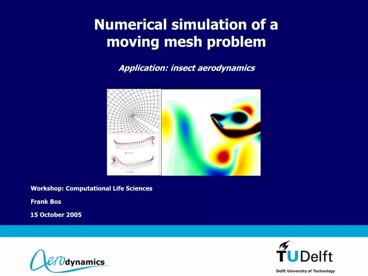
Numerical simulation of amoving mesh problem Application: insect aerodynamics Workshop: Computational Life Sciences Frank Bos
Overview Presentation • Problem description • Insect aerodynamics • Objectives • Material and methods • Numerical modelling • Validation and verification • Kinematic modelling • Results and discussions Introduction – Problem – Numerical modelling – Validation – Kinematic Modelling – Results – Conclusions
Background of insect flight (1/2) • Insect flight still not fully understood: • Quasi-steady aerodynamics could not predict unsteady forces • Experiments showed highly vortical flow • Vortex generation enhanced lift Leading Edge Vortex Introduction – Problem – Numerical modelling – Validation – Kinematic Modelling – Results – Conclusions
Background of insect flight (2/2) • Flow dominated by low Reynolds number: • Highly viscous and unsteady flow • At low Reynolds numbers flapping leads to efficient lift generation • Insects interesting to develop Micro Air Vehicles (intelligence, investigate hazardous environments) Introduction – Problem – Numerical modelling – Validation – Kinematic Modelling – Results – Conclusions
Problem Statement • Performance in insect flight is strongly influenced by wing kinematics. • Literature shows a wide range of different kinematic models. Main question What is the effect of different kinematic models on the performance in insect flight? Introduction – Problem – Numerical modelling – Validation – Kinematic Modelling – Results – Conclusions
Objectives • To develop an accurate numerical model for this challenging application. • Unravel unsteady aerodynamics of flapping insect aerodynamics. Procedure • Numerical modelling using general tools to solve Navier-Stokes equations. • Validation of the numerical model using static and moving cylinders. • Investigate influence of different wing kinematics on performance in hovering fruit-fly flight. Introduction – Problem – Numerical modelling – Validation – Kinematic Modelling – Results – Conclusions
Configuration set-up • Hovering fruit-fly (Drosophila Melanogaster) • Low Reynolds number = 110 • Low Mach number = 0.03 incompressible flow • 2-dimensional laminar flow Direct Numerical Simulation (DNS) • Airfoil = 2% thick ellipse • Different wing kinematics, derived from literature Introduction – Problem – Numerical modelling – Validation – Kinematic Modelling – Results – Conclusions
Material and methods • Finite volume based general purpose CFD solvers: Fluent (and HexStream) • Solve the Navier-Stokes equations: • Moving mesh using Arbitrary Lagrangian Eulerian (ALE) formulation: Introduction – Problem – Numerical modelling – Validation – Kinematic Modelling – Results – Conclusions
Mesh generation: Body conform in inner domain Re-meshing in outer domain at 25 diameters Body moves arbitrarily Motion restricting time step Numerical modelling Quarter of entire domain: Cells near the boundary: object Introduction – Problem – Numerical modelling – Validation – Kinematic Modelling – Results – Conclusions
Time step restrictions Rotation: Translation: N = number of cells on the surface = relative angular displacement y = relative linear displacement R = radius of cylinder ref = angular length of smallest cell yref = linear length of smallest cell Introduction – Problem – Numerical modelling – Validation – Kinematic Modelling – Results – Conclusions
Validation using moving cylinders Summarising: • All cells are optimal and moving • Mesh size = 50k and considered sufficient • Re-meshing occurs at 25 diameters • Validated for moving (rotating and translating) cylinders with literature • Timestep restriction due to interpolation in time When relative cell displacement < 10% then the corresponding time step leads results within 5% of literature. Extend this method to moving wings !!! Introduction – Problem – Numerical modelling – Validation – Kinematic Modelling – Results – Conclusions
Verification using moving wing Close-up at the Leading Edge: • Numerical model: • Conformal mapping: • 2% thick ellipse Time step dependence: Grid size dependence: fine Introduction – Problem – Numerical modelling – Validation – Kinematic Modelling – Results – Conclusions
Definition of motion parameters • 3D parameters: • Amplitude: • Angle of Attack: • Deviation: • 2D parameters: • Amplitude: x = Rgf / c • Angle of Attack: • Deviation: y = Rg q / c y x Rg = radius of gyration; c = averaged chord Introduction – Problem – Numerical modelling – Validation – Kinematic Modelling – Results – Conclusions
4 different kinematic models • Model 1: Harmonic • : cosine • : sine • : no ‘figure of eight’ • Model 2: Robofly • : ‘Sawtooth’ • : ‘Trapezoidal’ • : no ‘figure of eight’ • Model 3: Fruit-fly • : cosine • : Extra ‘bump’ • : ‘Figure of Eight’ • Model 4: Simplified Fruit-fly • : symmetrised • : symmetrised • : symmetrised • All Fruit-fly characteristics preserved Experiment: Introduction – Problem – Numerical modelling – Validation – Kinematic Modelling – Results – Conclusions
Matching kinematic models A reference is needed to make comparison of results between different models meaningfull Matching the quasi-steady lift of the cases to be compared Derived using 3D robofly Introduction – Problem – Numerical modelling – Validation – Kinematic Modelling – Results – Conclusions
Performance influence strategy • Compare complete Robofly with the fruit-fly models • Compare Robofly characteristics with harmonic model • Compare fruit-fly characteristics with harmonic model • Performance: • Investigate influence on lift, drag and performance • Glide ratio CL/CD is used as a first indication of performance • Look at vorticity! Introduction – Problem – Numerical modelling – Validation – Kinematic Modelling – Results – Conclusions
Comparison robofly and fruit-fly model Robofly and real Fruit-fly compared: • Robofly: mean lift 8% less than fruit-fly • Robofly: mean drag 80% more than fruit-fly • The symmetry less influence • Mean lift is well predicted, succesfull matching • Take a closer look at the force diagrams and vorticity Introduction – Problem – Numerical modelling – Validation – Kinematic Modelling – Results – Conclusions
Comparison different shapes Influence of different kinematic shapes w.r.t. harmonic model: Robofly Fruit-fly • Comparable mean lift coefficients • Mean drag is strongly affected ! • Robofly decreases performance, -25% to -30% • ‘bump’ in angle of attack increases performance considerably, 25%! • Deviation slightly decreases drag but strongly influences force variation! • Closer look at fruit-fly kinematics: ‘bump’ and deviation Introduction – Problem – Numerical modelling – Validation – Kinematic Modelling – Results – Conclusions
- ‘bump’ increases performance Harmonic Harmonic + ‘bump’ AOA • ‘bump’ decreases early angle of attack • Wing orientation high lift, low drag • ‘bump’ responsible for higher performance Introduction – Problem – Numerical modelling – Validation – Kinematic Modelling – Results – Conclusions
Deviation levels the forces • Deviation leads to changes in the effective angle of attack • Deviation is levelling forces • Early low peak is increased • Late high peak is decreased • Deviation causes more balanced force distributions Introduction – Problem – Numerical modelling – Validation – Kinematic Modelling – Results – Conclusions
Conclusions • Altough first order in time, accurate results were obtained with the model • The mean lift is comparable for all kinematic models. The mean lift deviates less than the mean drag. • Extra `bumb’ in angle of attack reduces drag considerably, thus increases performance • Deviation in fruit-fly levels the forces stability and control or more comfortable flight • Evidence was found that a fruit-fly uses the ‘bump’ to increase performance and the deviation to manipulate stability and control Introduction – Problem – Numerical modelling – Validation – Kinematic Modelling – Results – Conclusions
Recommendations • Use or develop higher order time discretisation methods • Investigate 3D effects • Varying broader parameter spectrum • Use other performance parameters, like work, required energy • Not only hovering, but also forward flapping flight may be interesting Introduction – Problem – Numerical modelling – Validation – Kinematic Modelling – Results – Conclusions
Cells in vortices, Re=150 Extra slides
Drag robofly 80% higher than fruit-fly Fruit-fly Robofly Large a in Roboflyleads to high drag and strong vortices Orientation wing leads to higher drag Possibly large influence of the large acceleration in amplitude and angle of attack (sawtooth and trapezoidal shapes) Introduction – Problem – Numerical modelling – Validation – Kinematic Modelling – Results – Conclusions
‘sawtooth’ increases drag Harmonic Harmonic + `sawtooth’ amp. • Sawtooth responsible for high drag • at the beginning ! High accel. • 2. Stronger vortices Introduction – Problem – Numerical modelling – Validation – Kinematic Modelling – Results – Conclusions
- ‘trapezoidal’ increases drag Harmonic Vortex shedding Harmonic + `trapezoidal’ angle of attack. • High drag: 48% increase • Wake capture of its LEV at t=0.6T • 2. LEV longer attached due to constant • angle of attack in Trapezoidal model Introduction – Problem – Numerical modelling – Validation – Kinematic Modelling – Results – Conclusions