Download
1 / 67
680 likes | 790 Views
EPI 5344: Survival Analysis in Epidemiology Time varying covariates March 25, 2014. Dr. N. Birkett, Department of Epidemiology & Community Medicine, University of Ottawa. Objectives. Introduce time varying covariates Methods of inclusion into Cox models SAS (computer) issues.

E N D
EPI 5344:Survival Analysis in EpidemiologyTime varying covariatesMarch 25, 2014 Dr. N. Birkett, Department of Epidemiology & Community Medicine, University of Ottawa
Objectives • Introduce time varying covariates • Methods of inclusion into Cox models • SAS (computer) issues
Introduction (1) • Does heart transplantation improve survival? • Epidemiological study with ID measures • Observational study (not an RCT) • Assume that transplant has no effect on survival • IDR = 1.0 • 800 candidates for transplant • 2 year follow-up • No losses • 50% of people get a transplant • Always occurs on their first anniversary of entering study • 25% of group die in first year • 25% of first year survivors die in second year
Introduction (2) Ignore transplant status
Introduction (3) Stratify by transplant status Transplant Done
Introduction (4) Stratify by transplant status NO Transplant Done
Introduction (5) • What is the observed IDR under this method of analysis? • Transplant ID = 0.133/yr • No transplant ID = 0.526/yr • IDR = 0.253 • Correct IDR = 1.0 STRONG BIAS Doing an RCT does NOT fix this issue as long as transplant isn’t done at time=0
Introduction (6) • How do we fix this? • No-one is at risk of dying with a transplant until the transplant has taken place • SO: • Accumulate PT (and events) to the non-transplant group until after a transplant occurs • Only accumulate PT (and events) to the transplant group after transplant occurs
Introduction (7) CORRECT WAY: No Transplant Done
Introduction (8) CORRECT WAY Transplant Done
Introduction (9) • What is the observed IDR under this method of analysis? • Transplant ID = 0.286/yr • No transplant ID = 0.286/yr • IDR = 1.0 • Correct IDR = 1.0 TIME VARYING COVARIATE Transplant status
Time Varying Covariates (1) • Exposures can change during follow-up • People stop/start smoking • BP increases • Air pollution varies from year to year • Hazard often depends more strongly on recent values than original exposure • Not always true • Can depend on • cumulative exposure • Lagged exposure • Produces non-proportional hazards (over all time) • Still proportional conditional on value of time varying exposure.
Time Varying Covariates (2) NOT PH over all time Before t*, HR = 1.0 After t*, HR* < 1.0 If we ignore the time of exposure and just treat these as two groups with PH, we get a biased estimate of the hazard ratio • A type of average of 1.0 and HR* (> HR*)
Time Varying Covariates (3) BUT: before t*, hazards are proportional after t*, hazards are proportional • The true impact of the exposure is HR* and only occurs after t* • Need an analysis approach to reflect this
Time Varying Covariates (4) • Is this hard to do? • YES and NO • Consider a situation where all subjects start off as ‘unexposed’ but at some time in the future, some people become exposed
Time Varying Covariates (5) Standard Cox Model Time Varying Cox Model Only change
Time Varying Covariates (6) • The theory really is this simple! • WHY? RISK SETS
Time Varying Covariates (7) • Likelihood function for Cox model is computed at each time point when an event occurs • Depends only on subjects “at risk” at the event time • RISK SET xij is the value of ‘x’ AT THE TIME of this event
Time Varying Covariates (8) Fixed covariates: xij is the same at all times Time varying covariates: Use the xij which corresponds to the event time of this risk set Keep going over all risk sets
Time Varying Covariates (9) • So why isn’t it simple to do this? • Practical Issues intrude!!!! • To fit a time varying covariate, SAS needs to know the value of the covariate for every risk set. • Need to compute a value of the covariate at the time of every event.
Proc Phreg programming (3) Example • 4 subjects • 2 get transplant at t=15 & t=25 • Want to include a time-varying covariate for transplant status. 4 risk sets at t=10, 20, 30, & 40
Time Varying Covariates (10) • Two ways to do this: • Include programming statements in ‘Proc Phreg’. • Re-structure the data set and use a different method of describing the model to SAS • Counting Process Input. • We’ll look at both ways. • Some things can only be done in the Phreg programming approach • Counting Process input has some strong benefits.
Proc Phreg programming (1) • SAS lets you include programme statements within PROC PHREG: proc phreg data=njb1; model surv*vs(0)=age sex x1; if (surv > 20) then x1 = 2; else x1 = 1; run;
Proc Phreg programming (2) • This code is processed once for each risk set • ‘surv’is the time when the risk set occurs • It is NOT the survival time for the subject • ‘x1’ is the value of the variable in the specific risk set under consideration. • Here, it is ‘1’ if the risk set occurs before time 20 but ‘2’ otherwise • File can get VERY BIG • Hard to de-bug your code
Standard PHreg analysis. Defines the ‘transplant’ status in the ‘data step’ using: if (dot = .) then trans = 0; else trans = 1;
Trans=1 a) Had a transplant b) Lived long enough to have a transplant
Hazard curves look something like this. Transplant Transplant time No Transplant In this interval, HR = 0 Overall HR is biased
Stanford Heart Transplant Study: with time varying effect For each event time, we need to define the transplant variable for every subject still in risk set trans = 0 no transplant by risk set time 1 transplant done on or before risk set time
SAS Code to create ‘trans’ and run analysis proc phreg data=stan; model surv1*dead(0)=plant surg ageaccept/ ties=exact; if (wait > surv1 or wait = .) then plant = 0; else plant = 1; run;
Counting Process Input (1) • Counting processes are a different way to look at survival • mathematically more powerful • essentially, each subject follows a ‘process’ • ‘count up’ the events they experience • can handle recurrent events • enhances modeling of exposure. • Don’t need to know all this to use SAS counting process style input.
Counting Process Input (2) • Data set needs to be restructured. • To-date • one record per subject • If covariate changes, coded in the record • need to use ‘phreg’ programming to define value at risk set. • New approach • one row per subject for each interval during which covariate is constant.
Counting Process Input (3) • Need to re-structure data file • Similar to piece-wise exponential • Follow-up time is dividing into intervals • For each subject, create a interval every time at least one time-varying covariate changes value • Each interval needs a record in the data set
Counting Process Input (3a) • Need to re-structure data file • Each interval needs a record in the data set • Need to code • Start of this interval • End of this interval • Outcome status at end of interval • Value of time varying covariate(s) during the interval • Values of fixed covariates, etc.
Counting Process Input (4) • Let’s use data from the Stanford Heart Transplant Study • the same data as before. • But, we only include transplant status • Ignore other variables for now. • Here, only one time varying covariate.
Re-structured data Original data
SAS Code to re-structure data DATA stanlong; SET allison.stan; plant=0; start=0; IF (trans=0) THEN DO; dead2=dead; stop=surv1; IF (stop=0) THEN stop=.1; OUTPUT; END; ELSE DO; stop=wait; IF (stop=0) THEN stop=.1; dead2=0; OUTPUT; plant=1; start=wait; IF (stop=.1) THEN start=.1; stop=surv1; dead2=dead; OUTPUT; END; RUN;
SAS Code for counting-process input analysis PROC PHREG DATA=stanlong; MODEL (start,stop)*dead2(0)=plant surg ageaccpt / TIES=EFRON; RUN; Identical to previous time-varying analysis
Time Varying Covariates (11) Types of time varying covariates • Internal (endogenous) • Change in the covariate is related to the behaviour of the subject. • Measurement requires subject to be under periodic examination • Blood pressure • Cholesterol • Smoking • More challenging for analysis • Often part of causal pathway
Time Varying Covariates (12) • External (exogenous) • Variables which vary independently of the subject’s normally biological processes. • The values do not depend on subject-specific information • Measurement does not require subject monitoring • Hourly pollen count
Time Varying Covariates (13) • Some pattern types • Non-reversible dichotomy • Transplant • Reversible dichotomy • Smoking • Drug use • Continuous variable • cholesterol
Time Varying Covariates (14) • Some issues • Need for valid measures for all subjects at all follow-up time • Missing data • ‘coarse’ measurement intervals • Imputation • Interpolation • Computationally intense • Reverse causation effects • Intermediate variables in the causal pathway
Time Varying Covariates (15) Some Logical fallacies • Can not use the future to predict the future! • Example #1 • Recruit a cohort of neonates • Age at entry = 0 for all subjects • Not useful as a predictor • Suggestion is made to use average age during follow-up to predict outcome • INVALID • Average age during follow-up depends on ‘future’ information • High average age is due to long survival
Time Varying Covariates (16) Intermediaries (Internal covariates) • RCT of anti-hypertensive treatment • Outcome: time to stroke • Main Q: Does drug rate of stroke • Model 1: ln(HR) = β1 (drug) • BUT, we measured BP on all subjects during follow-up. • Why not include this as a time-varying covariate?
Time Varying Covariates (17) Intermediaries (cont) • Model 1: ln(HR) = β1 (drug) • Model 2: ln(HR) = β1*(drug) + β2 BP(t) • Results • Model 1 β1: p < 0.001 • Model 2 β1*: p =0.6 WHY?