Download
1 / 38
410 likes | 576 Views
Eligibility Traces (ETs) Week #7. Introduction. A basic mechanism of RL. λ in TD( λ ) refers to an eligibility trace. TD methods such as Sarsa and Q-learning may be combined with ETs to obtain more efficient learning methods. Two different ways to view ETs: Forward view Backward view.

E N D
Introduction • A basic mechanism of RL. • λ in TD(λ) refers to an eligibility trace. • TD methods such as Sarsa and Q-learning may be combined with ETs to obtain more efficient learning methods. • Two different ways to view ETs: • Forward view • Backward view
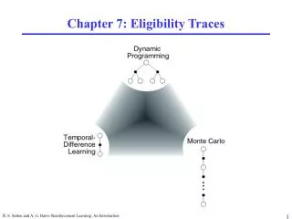
Forward View of ET • A more theoretical view: ETs are a bridge between TD and MC methods. • TD methods extended with ETs form a family with TD methods at one end and MC methods at the other.
ET: Definition Definition: An eligibility trace is a record to keep track of the extent to which a variable in an adaptive system deserves to be updated by the occurrence of a reinforcing event. Example: The event of how recently an action in a state is selected determines the extent of the eligibility of the value of the action in the relevant state to be updated.
n-Step TD Prediction • Value updates are based upon • the entire sequence of observed rewards, at one end (MC methods) and, • the next reward at the other end (TD methods). • Update rules using an intermediate number of observed rewards are called the n-step TD methods. • In this context, we call the latter TD methods using the next reward one-step TD methods.
Updates... from one end to the other where Rtis the complete return, T is the last time step of the episode andRt(n)is called thecorrected n-step truncated return.
On-line and off-line updating • The value estimates are updated with the above increment either immediately • Vt+1(s)=Vt(s)+ΔVt(s), (on-line updating), • or after the entire episode is over • (off-line updating)
Forward View of TD(λ) • Increments may also be established by any weighted combination of the i-step returns where the weights add up to 1. • Example:
Forward View... cont’d (2) • Another example: λ-return • with 0≤λ≤1. • The i-step return is given the ith largest weight (1-λ) λi-1.
Forward View... cont’d (3) • The λ-return algorithm ... • ... can also be expressed in the following way:
Forward View... cont’d (4) • λ-return as expressed here shows better that • the λ-return is a bridge between TD and MC methods, at two opposite ends, by the following two facts • with λ =0, the λ-return turns to TD methods • with λ =1, the λ-return turns to MC methods
Forward View ... Final word • Rather a theoretical view of the TD(λ). • An acausal view (i.e., return estimate Rtλ at time t is defined in terms of one or more future rewards rt+x, x∈N+); therefore hard to implement • The backward view more handy for implementation
Backward View of TD(λ) • A more mechanistic rather than theoretical view. • Causal • Associates each state (or action at a state) with a variable, the eligibility trace, that specifies how eligible the corresponding state (or action at a state) is for updates by the current reward.
Backward View of TD(λ) • The eligibility trace, denoted by et(s), of a state s is mathematically expressed as follows: • On each step, the eligibility trace, et(s), decays by γλ, and, if visited, its value is refreshed by incrementing by 1 where γ is the discount rate and λas introduced before is called the trace-decay parameter.
Backward View of TD(λ) • This kind of ET is called an accumulating trace to indicate that, at every visit of a state, the state’s eligibility trace accumulates then fades away with any time step it is not visited. • The reinforcing events are the moment-by-moment TD errors and may be mathematically expressed as follows: • Then the corresponding update becomes • Based on these update increments performed at each time step, the TD(λ) algorithm is given on next page:
Algorithm: TD(λ) • Initialize V(s) arbitrarily and e(s)=0, for all s ∈S • Repeat for each episode • Initialize s; • Repeat for each step of episode • a ← π(s) • Performa; observe r, and next state s’ • δ ←r+γV(s’)-V(s) • e(s)=e(s)+1 • For all s: • V(s)←V(s)+αδe(s) • e(s) ←γλe(s) • s ← s’ • Until s is terminal
Remarks • Backward view of TD(λ) is causal meaning that the state/action values are a function of past (.ie., not future) state/action values. • The past values are updated at each time step based on the current TD error depending on the state’s ET. • Special cases: • λ =0: et(s)=0 except for s=st → TD(0) method • λ =1: λ does not decay credit given to earlier states; hence each state receives credit based upon when it is visited. → MC method or TD(1) method.
Sarsa(λ) • ETs can be used to control an environment. • As usual, we need simply learn action values Qt(s,a) rather than state values Vt(s). As the relation of TD(λ) to TD(0), the version of the Sarsa algorithm with ETs is called Sarsa(λ), and the original version, from now on, one-step Sarsa. • The symbol et(s,a) denotes the eligibility trace for action a at state s, andδt =rt+1+γQt(st+1,at+1)-Qt(st,at) represents the update in action values.
Sarsa(λ)... Formulae • Further, the following formulae represent the action updates and eligibility traces in Sarsa, respectively:
Sarsa(λ)... Algorithm • Initialize Q(s,a) arbitrarily and e(s,a)=0, for all s,a • Repeat for each episode • Initialize s,a; • Repeat for each step of episode • Performa; observe r, and next state s’ • Choose a’ from s’ using policy derived from Q(e.g., ε-greedy) • δ ←r+γQ(s’,a’)-Q(s,a) • e(s,a)=e(s,a)+1 • For all s,a: • Q(s,a)← Q(s,a)+αδe(s,a) • e(s,a) ←γλe(s,a) • s ← s’; a←a’ • Until s is terminal
Q(λ) • Q(λ) is the off-policy RL method with ETs • Two versions of Q(λ) • Watkin’s Q(λ) • Peng’s Q(λ) • The essence of using ETs is; in order to end up with the optimal policy, to increment the values of states or state-action pairs at each time step on the basis of the extent to which it has received visits. • Looking at Sarsa(λ) algorithm, we observe that at each time step the γλ-decayed ET e(s) ore(s,a) weighting the error δt that adjusts the value of the state or state-action pair is or is not incremented depending upon whether or not the state or state-action pair is taken using the policy.
Q(λ) ... (2) • In the off-policy case, there is no problem as long as the state-action pair selections in the estimation and behavior policy are the same. • The problem starts at the point where the behavior policy branches away from the estimation policy. The first of the possible exploratory (i.e., non-greedy) actions in the behavior policy interrupts the sequence of action-response loop in the estimation policy and does not provide any correct subsequential experience on the estimation policy any more. • So, it is no longer usable after the first exploratory action to follow the behavior policy.
Watkin’s Q(λ) ...FW view • Watkin’s Q(λ) is just the same as TD(λ) with the only difference that the learning stops at whichever of the the first exploratory (i.e., non-greedy) action or the end of the episode occurs first. • To be exact, if at+n is the first exploratory action the longest backup is toward • where off-line updating is assumed.
Watkin’s Q(λ) ...BW view • From a mechanistic viewpoint, Watkin’s Q(λ) exploits ETs just the same as Sarsa(λ) with the only difference that the ETs are set to 0 whenever an exploratory (i.e., non-greedy) action is taken. • Formally, the trace update is expressed as follows:
Watkin’s Q(λ)... Algorithm • Initialize Q(s,a) arbitrarily and e(s,a)=0, for all s,a • Repeat for each episode • Initialize s,a; • Repeat for each step of episode • Performa; observe r and next state s’ • Choose a’ from s’ using policy derived from Q(e.g., ε-greedy) • a*←argmaxbQ(s’,b) (if a’ ties for the max, then a*=a’) • δ ←r+γQ(s’,a*)-Q(s,a) • e(s,a)=e(s,a)+1 • For all s,a: • Q(s,a)← Q(s,a)+αδe(s,a) • if a*=a’ then e(s,a) ←γλe(s,a) • else e(s,a) ← 0 • s ← s’; a←a’ • Until s is terminal
Peng’s Q(λ) ... Motivation • Watkin’s Q(λ) is not sufficiently effective if exploratory actions are taken frequently (i.e., ε high) since a sufficiently long sequence of experience or backups will not form, hence, learning may be only little faster than learning with one-step Q learning. • Peng’s Q(λ) is meant to handle this problem. • It is a mixture of Sarsa(λ) and Q(λ). • The key is that there is no distinction between the behavior and estimation policy up until the last action taken at which a greedy selection is preferred. • It should converge to an intermediate policy between Qπ and Q*. The more greedy the policy is made gradually the higher the probability is made for the policy to converge to Q*.
Replacing Traces • Sometimes a better performance may be obtained using the so-called replacing trace with the following trace updates: • With replacing traces the trace will never exceed 1 as opposed to accumulating traces which outperform accumulating traces in cases in which there is a good probability of taking a wrong action several consecutive times (see example 7.5 pp 186 & Fig. 7.18).
The start state is the left-most state and goal is the orange square. Rewards are zero except that for the action that accesses the goal that provides a +1. Imagine what happens when wrong is taken by the agent several times before right. wrong wrong wrong wrong wrong right right right right right +1 Example
With accumulating traces: At the end of the first episode, e(s,wrong)>e(s,right), although right is more recent, wrong is selected more frequently. At the receipt of the reward, this is likely to cause Q(s,wrong)>Q(s,right). This will not continue endlessly. Eventually as right is selected more frequently, the convergence will occur on right; but learning will slow down. wrong wrong right right right right +1 wrong wrong wrong right Example ...(2)
With replacing traces: This will not happen since the trace’s value will not accumulate but be replaced (i.e., the value of the trace will not be incremented by 1, but its highest value will be 1 whenever its relevant state is visited.) Hence, a recent right will have higher value than a wrong with several less recent visits. wrong wrong right right right right +1 wrong wrong wrong right Example ...(3)
Control Methods with Replacing Traces • Control methods may use replacing ETs. • Here, the ETs should be modified to involve action selections and distinguish between the action taken and those that are not. • The following reflects the necessary modification: • Testing this formula with the same example shows that this works even better.
Implementation Issues • Methods with ETs may seem to enhance the computational cost a lot since they require the computation of the ETs of every state (or, even more dramatically, every state-action pair). • Thank to the fastly decaying γλ factor of ETs, however, one can see that, for typical values of λ and γ, the ETs of only the recently visited states are significant. Those of almost all other states are almost always nearly zero. • Consequence: Sufficient to keep record of those states only with significant values of ETs!
Variable λ • An advanced topic; • Open to research especially on practical applications; • It involves allowing λ to vary in time (i.e., λ= λt). • An interesing way to vary λ would be to have it change as a function of states(i.e., λt= λ(st)). • How would you like to have λ(st) change then?
Variable λ • For those states whose values are believed to be known with high certainty should contribute to the estimate fully (meaning that the traces should be cut off for these states, λ near 0); • Others with highly uncertain value estimates should undergo a significant amount of adjustment, meaning a λ value closer to 1.
Forward View of Variable λ • The general definition of λ-return algorithm ... • ... can also be expressed in the following way:
Conclusions • MC methods are mentioned to have advantages in non-Markov tasks since they do not bootstrap. • Because ETs make TD methods like MC methods they are also advantageous in non-Markov tasks. • Methods with ETs require more computation than one-step methods, but in return they offer significantly faster learning, particularly when rewards are delayed by many steps. Hence, ETs are useful when data are scarce and cannot be repeatedly processed, as is the case in most on-line applications.
References • [1] Sutton, R. S. and Barto A. G., “Reinforcement Learning: An introduction,” MIT Press, 1998