Chapter 7: Eligibility Traces

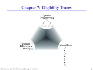
1. Chapter 7: Eligibility Traces R. S. Sutton and A. G. Barto: Reinforcement Learning: An Introduction

2. N-step TD Prediction • Idea: Look farther into the future when you do TD backup (1, 2, 3, …, n steps) R. S. Sutton and A. G. Barto: Reinforcement Learning: An Introduction

3. Mathematics of N-step TD Prediction • Monte Carlo: • TD: • Use V to estimate remaining return • n-step TD: • 2 step return: • n-step return: R. S. Sutton and A. G. Barto: Reinforcement Learning: An Introduction

4. Maximum error using n-step return Maximum error using V Learning with N-step Backups • Backup (on-line or off-line): • Error reduction property of n-step returns • Using this, you can show that n-step methods converge n step return R. S. Sutton and A. G. Barto: Reinforcement Learning: An Introduction

5. Random Walk Examples • How does 2-step TD work here? • How about 3-step TD? R. S. Sutton and A. G. Barto: Reinforcement Learning: An Introduction

6. A Larger Example • Task: 19 state random walk • Do you think there is an optimal n (for everything)? R. S. Sutton and A. G. Barto: Reinforcement Learning: An Introduction

7. Averaging N-step Returns One backup • n-step methods were introduced to help with TD(l) understanding • Idea: backup an average of several returns • e.g. backup half of 2-step and half of 4-step • Called a complex backup • Draw each component • Label with the weights for that component R. S. Sutton and A. G. Barto: Reinforcement Learning: An Introduction

8. Forward View of TD(l) • TD(l) is a method for averaging all n-step backups • weight by ln-1 (time since visitation) • l-return: • Backup using l-return: R. S. Sutton and A. G. Barto: Reinforcement Learning: An Introduction

9. l-return Weighting Function R. S. Sutton and A. G. Barto: Reinforcement Learning: An Introduction

10. Relation to TD(0) and MC • l-return can be rewritten as: • If l = 1, you get MC: • If l = 0, you get TD(0) Until termination After termination R. S. Sutton and A. G. Barto: Reinforcement Learning: An Introduction

11. Forward View of TD(l) II • Look forward from each state to determine update from future states and rewards: R. S. Sutton and A. G. Barto: Reinforcement Learning: An Introduction

12. l-return on the Random Walk • Same 19 state random walk as before • Why do you think intermediate values of l are best? R. S. Sutton and A. G. Barto: Reinforcement Learning: An Introduction

13. Backward View of TD(l) • The forward view was for theory • The backward view is for mechanism • New variable called eligibility trace • On each step, decay all traces by gl and increment the trace for the current state by 1 • Accumulating trace R. S. Sutton and A. G. Barto: Reinforcement Learning: An Introduction

14. On-line Tabular TD(l) R. S. Sutton and A. G. Barto: Reinforcement Learning: An Introduction

15. Backward View • Shout dt backwards over time • The strength of your voice decreases with temporal distance by gl R. S. Sutton and A. G. Barto: Reinforcement Learning: An Introduction

16. Relation of Backwards View to MC & TD(0) • Using update rule: • As before, if you set l to 0, you get to TD(0) • If you set l to 1, you get MC but in a better way • Can apply TD(1) to continuing tasks • Works incrementally and on-line (instead of waiting to the end of the episode) R. S. Sutton and A. G. Barto: Reinforcement Learning: An Introduction

17. Backward updates Forward updates Forward View = Backward View • The forward (theoretical) view of TD(l) is equivalent to the backward (mechanistic) view for off-line updating • The book shows: • On-line updating with small a is similar algebra shown in book R. S. Sutton and A. G. Barto: Reinforcement Learning: An Introduction

18. On-line versus Off-line on Random Walk • Same 19 state random walk • On-line performs better over a broader range of parameters R. S. Sutton and A. G. Barto: Reinforcement Learning: An Introduction

19. Control: Sarsa(l) • Save eligibility for state-action pairs instead of just states R. S. Sutton and A. G. Barto: Reinforcement Learning: An Introduction

20. Sarsa(l) Algorithm R. S. Sutton and A. G. Barto: Reinforcement Learning: An Introduction

21. Sarsa(l) Gridworld Example • With one trial, the agent has much more information about how to get to the goal • not necessarily the best way • Can considerably accelerate learning R. S. Sutton and A. G. Barto: Reinforcement Learning: An Introduction

22. Sarsa(l) Reluctant Walk Example • N states and two types of action right and wrong • When a wrong action, no reward and state not changed • Right action moves towards the goal • Reward +1 received when the terminal state reached Consider Sarsa(lambda) with eligibility traces R. S. Sutton and A. G. Barto: Reinforcement Learning: An Introduction

23. Sarsa(l) Reluctant Walk Example % Example 7.7 % reluctant walk - choosing right action moves you towards the goal % states are numbered from 1 to number_states clear all; close all; lambda=0.9; alpha=0.05; gamma=0.95; % rewards number_states=15; number_actions=2; number_runs=50; r=zeros(2,number_states); % first row are the right actions r(1,number_states)=1; % change alpha jjj=0; alpha_range=0.05:0.05:0.4; for alpha=alpha_range jjj=jjj+1; all_episodes=[]; for kk=1:number_runs S_prime(1,:)=(1:number_states); S_prime(2,:)=(1:number_states); % generate a right action sequence right_action=(rand(1,number_states)>0.5)+1; % next state for the right action for i=1:number_states S_prime(right_action(i),i)=i+1; end % eligibility traces e=zeros(number_actions,number_states+1); Qsa=rand(number_actions,number_states); Qsa(:,number_states+1)=0; num_episodes=10; t=1; % repeat for each episode for episode=1:num_episodes epsi=1/t; % initialize state s=1; R. S. Sutton and A. G. Barto: Reinforcement Learning: An Introduction

24. Sarsa(l) Reluctant Walk Example % chose action a from s using epsilon greedy policy chose_policy=rand>epsi; if chose_policy [val,a]=max(Qsa(:,s)); else a=ceil(rand*(1-eps)*number_actions); end; % repeat for each step of episode episode_size(episode)=0; path=[]; random=[]; while s~=number_states+1 epsi=1/t; % take action a, observe r, s_pr s_pr=S_prime(a,s); % chose action a_pr from s_pr using epsilon greedy policy chose_policy_pr=rand>epsi; [val,a_star]=max(Qsa(:,s_pr)); if chose_policy_pr random=[random 0]; a_pr=a_star; else a_pr=ceil(rand*(1-eps)*number_actions); random=[random 1]; end; % reward if s_pr==number_states+1 r=1; else r=0; end; delta=r+gamma*Qsa(a_pr,s_pr)-Qsa(a,s); % eligibility traces e(a,s)=e(a,s)+1; % Sarasa lambda algorithm Qsa=Qsa+alpha*delta*e; e=gamma*lambda*e; s=s_pr; a=a_pr; episode_size(episode)=episode_size(episode)+1; path=[path s]; t=t+1; end; %while s end; R. S. Sutton and A. G. Barto: Reinforcement Learning: An Introduction

25. Sarsa(l) Reluctant Walk Example all_episodes=[all_episodes; episode_size]; end; % kk last_episode=cumsum(mean(all_episodes)); all_episode_size(jjj)=last_episode(num_episodes); end; % alpha episode_size=mean(all_episodes); plot([0 cumsum(episode_size)],(0:num_episodes)); xlabel('Time step'); ylabel('Episode index'); title('Eligibility traces-SARSA random walk 15 states learning rate with eps=1/t, lambda=0.9'); figure(2) plot(alpha_range, (all_episode_size)); xlabel('Alpha'); ylabel('Number of steps for 10 episodes'); title('Eligibility traces-SARSA random walk 15 states learning rate with eps=1/t, lambda=0.9'); figure(3) plot( episode_size(1:num_episodes)) xlabel('Episode index'); ylabel('Episode length in steps'); title('Eligibility traces-SARSA random walk 15 states learning rate with eps=1/t, lambda=0.9'); R. S. Sutton and A. G. Barto: Reinforcement Learning: An Introduction

26. Sarsa(l) Reluctant Walk Example • Eligibility traces with alpha> 0.5 is unstable R. S. Sutton and A. G. Barto: Reinforcement Learning: An Introduction

27. Sarsa(l) Reluctant Walk Example • Learning rate in eligibility traces, alpha=0.4 R. S. Sutton and A. G. Barto: Reinforcement Learning: An Introduction

28. Three Approaches to Q(l) • How can we extend this to Q-learning? • If you mark every state action pair as eligible, you backup over non-greedy policy • Watkins: Zero out eligibility trace after a non-greedy action. Do max when backing up at first non-greedy choice. R. S. Sutton and A. G. Barto: Reinforcement Learning: An Introduction

29. Watkins’s Q(l) R. S. Sutton and A. G. Barto: Reinforcement Learning: An Introduction

30. Peng’s Q(l) • Disadvantage to Watkins’s method: • Early in learning, the eligibility trace will be “cut” (zeroed out) frequently resulting in little advantage to traces • Peng: • Backup max action except at end • Never cut traces • Disadvantage: • Complicated to implement R. S. Sutton and A. G. Barto: Reinforcement Learning: An Introduction

31. Naïve Q(l) • Idea: is it really a problem to backup exploratory actions? • Never zero traces • Always backup max at current action (unlike Peng or Watkins’s) • Is this truly naïve? • Works well is preliminary empirical studies What is the backup diagram? R. S. Sutton and A. G. Barto: Reinforcement Learning: An Introduction

32. Comparison Task • Compared Watkins’s, Peng’s, and Naïve (called McGovern’s here) Q(l) on several tasks. • See McGovern and Sutton (1997). Towards a Better Q(l) for other tasks and results (stochastic tasks, continuing tasks, etc) • Deterministic gridworld with obstacles • 10x10 gridworld • 25 randomly generated obstacles • 30 runs • a = 0.05, g = 0.9, l = 0.9, e = 0.05, accumulating traces From McGovern and Sutton (1997). Towards a better Q(l) R. S. Sutton and A. G. Barto: Reinforcement Learning: An Introduction

33. Comparison Results From McGovern and Sutton (1997). Towards a better Q(l) R. S. Sutton and A. G. Barto: Reinforcement Learning: An Introduction

34. Convergence of the Q(l)’s • None of the methods are proven to converge. • Much extra credit if you can prove any of them. • Watkins’s is thought to converge to Q* • Peng’s is thought to converge to a mixture of Qp and Q* • Naïve - Q*? R. S. Sutton and A. G. Barto: Reinforcement Learning: An Introduction

35. Eligibility Traces for Actor-Critic Methods • Critic: On-policy learning of Vp. Use TD(l) as described before. • Actor: Needs eligibility traces for each state-action pair. • We change the update equation: • Can change the other actor-critic update: to to where R. S. Sutton and A. G. Barto: Reinforcement Learning: An Introduction

36. Replacing Traces • Using accumulating traces, frequently visited states can have eligibilities greater than 1 • This can be a problem for convergence • Replacing traces: Instead of adding 1 when you visit a state, set that trace to 1 R. S. Sutton and A. G. Barto: Reinforcement Learning: An Introduction

37. Replacing Traces Example • Same 19 state random walk task as before • Replacing traces perform better than accumulating traces over more values of l R. S. Sutton and A. G. Barto: Reinforcement Learning: An Introduction

38. Why Replacing Traces? • Replacing traces can significantly speed learning • They can make the system perform well for a broader set of parameters • Accumulating traces can do poorly on certain types of tasks Why is this task particularly onerous for accumulating traces? R. S. Sutton and A. G. Barto: Reinforcement Learning: An Introduction

39. Sarsa(l) Reluctant Walk Example • Replacing traces delta=r+gamma*Qsa(a_pr,s_pr)-Qsa(a,s); % replacing traces % e(:,s)=0; e(a,s)=1; % Sarasa lambda algorithm Qsa=Qsa+alpha*delta*e; e=gamma*lambda*e; R. S. Sutton and A. G. Barto: Reinforcement Learning: An Introduction

40. Sarsa(l) Reluctant Walk Example • Replacing traces R. S. Sutton and A. G. Barto: Reinforcement Learning: An Introduction

41. More Replacing Traces • Off-line replacing trace TD(1) is identical to first-visit MC • Extension to action-values: • When you revisit a state, what should you do with the traces for the other actions? • Singh and Sutton say to set them to zero: R. S. Sutton and A. G. Barto: Reinforcement Learning: An Introduction

42. Implementation Issues • Could require much more computation • But most eligibility traces are VERY close to zero • If you implement it in Matlab, backup is only one line of code and is very fast (Matlab is optimized for matrices) R. S. Sutton and A. G. Barto: Reinforcement Learning: An Introduction

43. Variable l • Can generalize to variable l • Here l is a function of time • Could define R. S. Sutton and A. G. Barto: Reinforcement Learning: An Introduction

44. Conclusions • Provides efficient, incremental way to combine MC and TD • Includes advantages of MC (can deal with lack of Markov property) • Includes advantages of TD (using TD error, bootstrapping) • Can significantly speed learning • Does have a cost in computation R. S. Sutton and A. G. Barto: Reinforcement Learning: An Introduction

45. Something Here is Not Like the Other R. S. Sutton and A. G. Barto: Reinforcement Learning: An Introduction