Download
1 / 55
550 likes | 563 Views
Perceptual Organization of Contours. James Elder Centre for Vision Research York University Toronto, Canada. Edge perception Contour perception Neural coding. Outline. Edge Perception. Collaborators: Sherry Trithart Dmitri Beniaminov Yaniv Morgenstern.

E N D
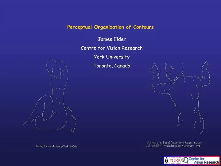
Perceptual Organization of Contours James Elder Centre for Vision Research York University Toronto, Canada
Edge perception Contour perception Neural coding Outline
Edge Perception Collaborators: Sherry Trithart Dmitri Beniaminov Yaniv Morgenstern
Linear Filters Underlying Edge Detection • Edge detection algorithms based on Gaussian derivative filters (Koenderink 84, Young 87, Parent & Zucker 89, Elder & Zucker 98, Lindeberg et al 98, etc.): • Is this how the human visual system detects edges?
500 ms 500 ms 200 ms Until Response Edge Detection Experiment
Classification Image Methodology • Beard & Ahumada, 1998; Murray et al, 2002 Response Y N Y Stimulus N
Example Stimulus Raw Classification Image Smoothed Classification Image X Profile Y Profile Gaussian Derivative Model Data Data Model Model -4 -2 0 2 4 -20 -10 0 10 20 Horizontal Position (deg) Vertical Position (deg) Example Observer: Low Noise Contrast (4.3%)
Cornsweet Edges Illusory Contours Mach Bands Some Demonstrations
T D T D 1600 T D 1400 1200 Response Time (msec) 1000 T D 800 600 0 5 10 15 Number of Distractors Reversing contrast leads to serial search (p<.00003) 1600 1400 1200 Response Time (msec) 1000 800 600 0 5 10 15 Number of Distractors
Contrast Blur Closure What cues determine our perception of shadows? In general, how do we classify contours?
1 5 3 2 4 Edge Taxonomy 1. Occlusion Edge 2. Reflectance Edge 3. Cast Shadow Edge 4. Attached Shadow Edge 5.Highlight Edge
Experiment 1. Edge Classification with Unrestricted Viewing • Purpose: • To estimate the incidence of each edge class in natural images • To provide baseline data for Expt 2. • Methods: • 60 images, 10 edges/image: 600 sample edge points in random order • 7 experienced observers
Results: Estimated incidence of edge classes in natural images
Means of Conditional Likelihood Distributions p(cue| edge class)
Detection is finely tuned to edges Gaussian derivative model accounts well for edge detection. Edges are (essentially) complete. Local cues (blur, contrast) important for classification. But purely local cues are inadequate Edge Perception: Main Observations
Contour Perception Collaborators:Rick Goldberg Leigh Johnston Amnon Krupnik Aaron Clarke
(Wertheimer, 23) Proximity Good Continuation Similarity Three Gestalt Principles Relevant to Contours Max Wertheimer
Proximity Good Continuation Similarity Three Gestalt Laws of Perceptual Organization
Correlational (co-occurence) statistics relate tangents regardless of their origin. • Contour set statistics (Geisler et al., 01) relate tangents regardless of their position along the contour. • Contour sequence statistics (Elder & Goldberg, 98, 02) relate only successive tangents along the contour. Which statistics are most relevant to contour grouping?
The one-dimensionality of contours imposes an ordering on the local elements of a curve. This property is essential for defining higher-order properties of contours, e.g. curvature, closure, concavity, convexity. One-Dimensionality of Contours
Model contours as Markov chains: assume long-range statistics completely determined by local statistics. Markov Chain Model
li1 lj1 r li2 lj2 ij t t i j Ecological Statistics of Natural Contours (JOV 02)
1 10 Data Power Law Model Simulated Noisy Power Law 0 10 -1 10 -2 10 -3 10 -4 10 -3 -2 -1 0 1 2 3 4 5 Proximity: Contour Likelihood Distribution p(Gap) log(Gap)
Quantitative Model of Proximity Dot lattice experiment (Oyama, 61)
Correlational statistics (Sigman et al.): b = 0.6 Contour set statistics (Geisler et al.): b = 1.44 Contour sequence statistics (Elder & Goldberg): b = 2.92 Contour sequence statistics (Clarke & Elder): b = 2.79 Power laws for proximity
What is the most natural scheme for encoding good continuation cues?
Theory 1. Perceptual organization is a general, bottom-up process that precedes scene recognition (e.g. Kanizsa 79) Theory 2. Perceptual organization is influenced by higher-level objectives, prior knowledge and specific context (e.g. Rock 83, Cavanagh 91). Using Prior Knowledge in Perceptual Organization
Using Higher Level Objectives to Tame the Complexity of Perceptual Organization
Contour Grouping with Prior Models (Elder, Krupnik & Johnston, PAMI 2003) • Grouping Cues • Proximity • Good Continuation • Luminance Similarity • Object cues: • Distance between tangent and model • Angle between tangent and model • Distance between tangent and nearest neighbouring tangent on dark side • Intensity on dark side of tangent
Posterior Prior Statistical Power of Object Cues
Geomatics applications (CCRS): Computing bounding contours of terrain features from satellite imagery
Example Result • Tested on 7 new lakes from IKONOS data • Average 41% improvement in accuracy over GIS data • Compared with performance of 8 human experts • Algorithm performed at the level of a human geomatics mapping expert Human Algorithm
Statistical cue integration based on ecological statistics Ecological tuning of human perceptual organization system Statistical integration of contextual priors Contour Perception: Main Points
Neural Coding Collaborators:Simon Prince Stephen David (Berkeley) Jack Gallant (Berkeley)
3 5 m s 4 9 m s 6 3 m s 7 7 m s 9 1 m s 1 0 5 m s Spatial Reverse Correlation
3 5 m s 4 9 m s 6 3 m s 7 7 m s 9 1 m s 1 0 5 m s Phase-separated Fourier-domain reverse correlation
3 2 1 0 -1 -2 -3 gradient direction tangent bundle representation stimulus local pooling gradient magnitude Constructing the tangent bundle representation
C O M P L E X C E L L O T H E R S I M P L E C E L L O r i e n t a t i o n t u n e d r e c e p t i v e f i e l d O r i e n t a t i o n t u n e d r e c e p t i v e M o r e e x o t i c c e l l r e s p o n s e s w i t h d i s t i n c t s p a t i a l a r e a s f i e l d , r e s p o n d s t o c o n t o u r s o f c a n a l s o b e d e s c r i b e d , s u c h r e s p o n d i n g t o e d g e s o f d i f f e r e n t e i t h e r p o l a r i t y r e g a r d l e s s o f a s s e l e c t i v i t y f o r t h i s c u r v e d p o l a r i t y . p o s i t i o n . e d g e s e c t i o n . What cell responses can the tangent bundle represent?
tangent bundle representation . . . . . . time cell response (spikes/sec) . . . . . . time Reverse correlation on the tangent bundle
7 m s 2 1 m s 3 5 m s 4 9 m s 6 3 m s 7 7 m s 9 1 m s 1 0 5 m s 1 1 9 m s 1 3 3 m s Example V1 Receptive Field 2 r 3 0 5 , r = 0 . 3 0 9 1 2