Download
1 / 22
220 likes | 363 Views
Optimization of Global Chassis Control Variables. Josip Kasać*, Joško Deur*, Branko Novaković*, Matthew Hancock**, Francis Assadian** * University of Zagreb, Faculty of Mech. Eng. & Naval Arch., Zagreb, Croatia (e-mail: josip.kasac@fsb.hr, josko.deur@fsb.hr, branko.novakovic@fsb.hr).

E N D
Optimization of Global Chassis Control Variables Josip Kasać*, Joško Deur*, Branko Novaković*, Matthew Hancock**, Francis Assadian** * University of Zagreb, Faculty of Mech. Eng. & Naval Arch., Zagreb, Croatia(e-mail: josip.kasac@fsb.hr, josko.deur@fsb.hr, branko.novakovic@fsb.hr). ** Jaguar Cars Ltd, Whitley Engineering Centre, Coventry, UK (e-mail: fassadia@ford.com, mhancoc1@jaguar.com).
Introduction • Introduction of new actuators- active rear steering (ARS), active torque vectoring differential (TVD), active limited-slip differential (ALSD),offersnew possibilities of improving active vehicle stability and performance • However, the control system becomes more complex (Global Chassis Control = GCC),which calls for application of advanced controller optimization methods • Benefits of using the nonlinear open-loop optimization: • assessment on the degree of GCC improvement achieved by introducing different actuators; • gaining an insight on how the state controller can be extended by feedforward and/or gain scheduling actions to improve the performance. • In this paper a gradient-based algorithm for optimal control of nonlinear multivariable systems with control and state vectors constraints is proposed • GCC application -double lane change maneuver executed by using control actions of active rear steering and active rear differential actuators.
Optimal control problem formulation • Find the control vector u(t) that minimizes the cost function Time-dicretization • subject to the nonlinear MIMO dynamics process equations Euler time-dicretization • with initial and final conditions of the state vector • subject to control & state vector inequality and equality constraints
Extending the cost function with constraints-related terms Basic cost function defined above Penalty for final state condition Weighting factors Penalty for inequality constraints Penalty for equality constraints Final problem formulation
Comparison with nonlinear programming based algorithms • Penalty functions: • Plant equation constraints: • Nonlinear programming approach: • Advantage vs. Nonlinear Programming based algorithms: Process equations constraints (ODE) are not included in the total cost function as equality constraints • The control and state vectors are treated as dependent variables, thus leading to backward in time structure of algorithm similar toBPTT algorithmfrom NN
Exact gradient calculation • Implicit but exact calculation of cost function gradient - chain rule for ordered derivatives • BPTT algorithm – time generalisation of BP algorithm
Modified gradient algorithm - convergence speed-up • The gradient algorithm with the constant convergence coefficient and a linear gradient is characterized by a slow convergence. • Small value of the gradient near the optimal solution is the main reason for the slow convergence. • a “sliding-mode”-based modification of the gradient algorithm • provides a stronger influence of the gradient near the optimal solution, and better convergence
Active Front d x Steering f D = t T 0 f y t T 2 1 f T D Central T i b c Power Differential Plant U V l CoG State r Active Rear Variables Steering T d r r c Rear D T Differential r x y 3 4 z t / 2 t / 2 Definition of vehicle dynamics quantities
1. State-Space Subsystem • 1.1 Longitudinal, lateral, and yaw DOF Fxi,Fyi,- longitudinal and lateral forces M- vehicle mass, Izz- vehicle moment of inertia, b - distance from the front axle to the CoG, c - distance from the rear axle to the CoG, t - track U, V - longitudinal and lateral velocity, r - yaw rate, X,Y - vehicle position in the inertial system ψ - yaw angle
1.2 The wheel rotational dynamics j- rotational speed of the i-th wheel, Fxti - longitudinal force of the i-th tire, Ti - torque at the i-th wheel, Iwi- wheel moment of inertia, R - effective tire radius. • 1.3 Delayed total lateral force (needed to calculate the lateraltire load shift): • 1.4 The actuator dynamics: - rear wheel steering angle, - rear differential torque shift, - actuator time constants.
2. Longitudinal Slip Subsystem 3. Lateral Slip Subsystem 4. TireLoad Subsystem l - wheelbase hg - CoG height 5. Tire Subsystem μ- tire friction coefficient B, C,D - tire model parameters
6. Rear Active Differential Subsystem ΔTr - differential torque shift control variable, Ti - input torque (driveline torque) and Tb - braking torque • Active limited-slip differential (ALSD): • Torque vectoring differential (TVD):
GCC optimization problem formulation • Nonlinear vehicle dynamics (process) description • Control variables (to be optimized): r(ARS) and Tr(TVD/ALSD) • Other inputs (driver’s inputs): f • State variables: U, V, r, i(i = 1,...,4), , X, Y • Cost functions definitions Reference trajectory • Path following(in external coordinates): • Control effort penalty: • Different constraints implemented: • control variable limit: • vehicle side slip angle limit: • boundary condition on Y and dY / dt:
Example: Double line change maneuver (22 m/s, =1) Reference trajectory for next optimizations • Front wheel steering optimization results for asphalt road ( = 1)
Optimization results for different actuators (=0.6) ARS+TVD ARS TVD ALSD • ARS and TVD gives comparable results; no advantage of combined ARS/TVD (except for lower control effort); ALSD less effective due to lack of oversteer generation
Optimization results for different actuators (=0.3) ARS+TVD ARS TVD ALSD • At low- surface the lateral optimizer limits lateral acceleration to stabilize vehicle; as a result trajectory tracking is worsen
Conclusions • A back-propagation-through-time (BPTT) exact gradient method for optimal control has been applied for control variable optimization in Global Chassis Control (GCC) systems. • The BPTT optimization approach is proven to be numerically robust, precise (control variables are optimized in 5000 time points), and rather computationally efficient • Recent algorithm improvement: • numerical Jacobians calculation • implementation of higher-order Adams methods • The future work will be directed towards: • use of more accurate tire model • introduction of a driver model for closed-loop maneuvers • model extension with roll, pitch, and heave dynamics • implementation of different gradient methods for convergence speed-up