Download
1 / 40
400 likes | 520 Views
Study of a bi-dimensional variational assimilation for soil moisture initialization in the mesoscale NWP model ALADIN. Gianpaolo BALSAMO, François BOUYSSEL, Jöel NOILHAN. ELDAS First pro g ress meetin g – KNMI De Bilt 12-13 December 2002. Plan of the presentation. INTRODUCTION

E N D
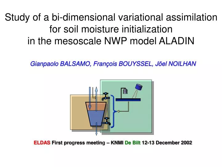
Study of a bi-dimensional variational assimilation for soil moisture initialization in the mesoscale NWP model ALADIN Gianpaolo BALSAMO, François BOUYSSEL, Jöel NOILHAN ELDAS First progress meeting– KNMIDe Bilt12-13 December 2002
Plan of the presentation • INTRODUCTION • The NWP context • The land surface scheme • The importance of soil moisture (an exemple) • LAND SURFACE ASSIMILATION • The techniques considered: optimum interpolation, variational • Comparison on 1D study • 2D-VAR ANALYSIS of SOIL MOISTURE • The implementation on a 3D model • Validation of the 2D-VAR assumptions • Optimization • ASSIMILATION EXPERIMENTS • Results and perspectives
ARPEGE:Global spectral stretched model 20 to 200 km, 41 levels (1 hPa) , 4 runs/day (96h) 4D-Var (T107, T161) : 6h assimilation cycle ALADIN-France:LAM, coupled to ARPEGE 9.5 km, 41 levels (1 hPa), 4 runs/day (48h) ALADIN LAM: 7 coupling domains Forecasts available on 14 integration domains (16km 7km) Unstretched ARPEGE: Global spectral regular model 66 km, 41 levels (1 hPa) 1 run/day (72h) 4D-Var (T107, T107) 6h assimilation cycle Operational NWP models AROME project: LAM over France, NH,2 km Own analysis system Operational in 2008
Surface Parameterization scheme (ISBA) Operational version: Noilhan & Planton (1989), Noilhan & Mahfouf (1996), Bazile (1999), Giard & Bazile (2000) Water Energy Analysis surface temperature mean soil temperature superficial soil water content total soil water content ~1-2 h ~1-2 d ~6-12 h ~10 d Research versions : interactive vegetation module (Calvet et al. 1998), sub grid-scale runoff and sub-root layer (Boone et al 1999), explicit 3-layers snow scheme (Boone & Etchevers 2001)
Importance of Soil Moisture in mesoscale NWP • Mean soil moisture distributes LE and H surface fluxes (Bowen ratio) • Affect PBL evolution • Mean soil moisture has a long time-scale memory (several weeks) Problems: • No regular observation of soil moisture • High resolution spatial variability of surface parameters Idea: • Use indirect observations (T2m, RH2m) (Coiffier et al. 1987, Mahfouf 1991) • A global surface analysis has been implemented for ARPEGE (Bouttier et al. 1993, Giard and Bazile, 2000) using an Optimum Interpolation technique • Initial soil moisture in ALADIN-France (interpolated from ARPEGE) • Correlation means improvements are possibles using Hi-res network
Test the 2m model biases under clear sky conditions on june 2000, 13th-18th Evalutation of 2m model errors is performed with the aid of Hi-res observations network Correlation of T2m errors & Soil moisture peaks Wet T2m) RMSE ~ 2°C -1°C< BIAS < 1°C RH2m) RMSE ~ 15% -5%< BIAS < 10% Dry heterogeneity of soil moisture (low realism)
Optimum interpolation of T2m and HU2m using SYNOP observations • Correction of surface parameters (Ts, Tp, Ws, Wp) using 2m increments between analysed and forecasted values Model forecast Analysis Obs Initialization of prognostic surface parametersoperational global surface analysis(Coiffier 1987, Mahfouf 1991, Bouttier 1993, Giard and Bazile 2000) • Sequential analysis (every 6h)
Callies et al. (1998), Rhodin et al. (1999), Bouyssel et al. (2000), Hess (2001), Balsamo et al. (2002) Formalism: Gradient of the cost function : General case : minimisation problem solved using an interative algorithm (TL/AD) TL hypothesis : H(x+dx) H(x) + H.dxFinite differences Variational surface analysis: 2D-VAR (z,t)
Advantages OI is linked to BLUE Many NWP centers use OI (ECMWF, Météo-France, HIRLAM, etc.) Based on a large statistics (Montecarlo) Drawbacks Tuning of the OI coefficients Reduced Portability Only averaged properties could be taken into account Based on 2m analysis Assimilation of 2m data by mean of Optimal Interpolation Assimilation of 2m data by mean of Variational approach • Advantages • VAR is linked to BLUE • Use observations at right time • Temporal consistency on the assimilation window • Keeps count of dynamics and physiography implicitely • Drawbacks • Computational cost • Coding of TL/AD (if linearisation is not allowed) • Based on 2m analysis
1D study on MUREX experiment Comparison of 2D-VAR and OI analyses on MUREX experiment for the year 1995 (Bouyssel 2001) • Minimisation of the cost function is obtained by TL/AD method applied on 1D model • Better results are obtained by the 2D-VAR when compared to the OI
3D study of 2D-VAR using finite differences • A linear estimate of observation operator is evaluated on every grid point with a finite difference method (Hess, 2001) Wpvegetation Wsbare ground
Forecast (6h or 24h) Wp W’p 3D study of 2D-VAR: formalism From a perturbation of the initial total soil moisture Wpa = Wpb + BHT(HBHT + R)-1(y - H(xb))
3D study of 2D-VAR: the main hyphoteses • Two main hyphotheses has to be validated • TL(linearity) • 2D(horizontal decoupling)
TL hypothesis B) A) Considering a real situation (16062000 at 12UTC), a sensitivity test on initial soil moisture is run under different atmospheric conditions T’2m T2m B) T’2m T2m A)
Calculate the H matrix term [K / m ] and compare it with the satellite image 20000616 at 12 UTC TL hypothesis (II)
Solutions for non-linearities of the observation operator Two ways to treat non-linearities • MASKING • Choice of masking criteria • efficient with no increase of cost but sub-optimal • OPTIMIZATION OF PERTURBATION • Choice of 2D shape • Choice of amplitude • Number of perturbations
Masking It has been considered a simple ON-OFF masking |Model Fields Threshold | Total Cloud Cover (fraction) 0.05Convective Cloud Cover (fraction) 0.05 Stratiform Precipitation (mm) 0.01Convective Precipitation (mm) 0.0110m Wind velocity (fraction of G) 0.10 or <0.05 ms-1Snow depth (m) 0.05Water frozen in soil (mm) 0.05Solar Radiation Flux (fraction of G) 0.01 or <1.0 Wm-2 2D-Var |Model Fields Threshold | Min solar time duration J_min 6 hMax wind velocity Vmax 10 ms-1Max precipitation P_max 0.3 mmMin evaporation E_min 0.001 mmMax soil ice W_imax 5.0 mm OI
Comparison of 2D-VAR and OI A comparison with OI (Gain Matrix and OI coefficients) is useful to point out some properties of the variational approach • masking of low sensitivity grid-points (coherence of masked areas) • dependency from radiation rather than vegetation • Evaluation of the overall correction of the OI ( ) OI 2D-Var Veg. cover (%) Radiation (W/m2)
2D hypothesis The 2D hypothesis is validated with simulated observations on a real situation From a prescribed initial error Wp Analysis error The 6-h forecast errors on T2mand RH2m
Solutions for non-linearities of the observation operator Two ways to treat non-linearities • MASKING • Choice of masking criteria • efficient with no increase of cost but sub-optimal • OPTIMIZATION OF PERTURBATION • Choice of 2D shape • Choice of amplitude • Number of perturbations
wp wpmed x x x x x Choice of 2D-shape for perturbation • Coherent • Random • Conditional • Chess-type
x x Chess-type perturbation perturbation(s) every 10 km perturbation(s) every 50 km
Number of perturbations. 2D hypothesis (II) 1 2 10 perturbation(s) every 10 km 10 perturbations every 50 km
Number of perturbations. 2D hypothesis (III) 1 2 10 perturbation(s) every 10 km 10 perturbations every 50 km
x Optimized setup for the 2D-VAR on ALADIN • Double Chess-typeno masking • Perturbation amplitude 20% of SWI[0,1] • Model forecast error (B) 5-10% of SWI[0,1] • Assimilation time window 24-h (obs. every 6-h)
Balsamo et al. (2002) Habets et al. (1999) 2D-VAR ALADIN compared to SIM off-line A 2D-VAR assimilation cycle is performed to analyse the soil moisture using real observations. A realistic soil moisture provided by a hydrological coupled model (SAFRAN-ISBA-MODCOU) forced by observations (Prec, Rad) is used for comparison.
T2m OI 2D VAR A more realisticsoil moisture is combined with forecast improvements HU2m 2D-VAR ALADIN compared to operational OI analysis
Conclusions • Improve the understanding of feedback mechanism in soil moisture analysis • Develop 2D-Var for assimilation of soil moisture • Compare different initialisations (OI, 2D-Var, off-line) • First validation test (25 days assimilation T=24h) Perspectives • Extensive validation and application in the frame of ELDAS • Inclusion of other observations ( TSIR, TBMO, Prec, Rad) • Satellite-measured radiation (MSG, AQUA, SMOS, …) • Three open questions:
The direct method (MUREX and other field site experiments) + Direct calculations (no overestimate of correlations) - Local estimate (non representative). The Montecarlo method (used for the operational analysis OI) + Easy to implement - Overestimation - Sensitivity to the choice of perturbation The NMC method + Independent sampling - Evaluation of forecast system errors (analysis + forecast) The ensemble method + Promising for an estimate of model errors (independent and realistic) (provided the surface analysis is swithched off). How to characterize forecast/model errors ?
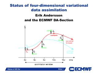
10 days 5 days 48 h 24 h 12 h 6 h t t0 length of assimilation window (6 to 240 hours?)
Daily statistics efficiency, r2 Monthly statistics efficiency,correlation squared,ratio (sim/obs) A. Boone (2002)
Boundary layer scheme w Soil Moisture assimilation: the ‘off-line’ and ‘coupled’ methods The LDAS/GLDAS approach The ELDAS approach Sat. data Observed Precip, Rad. Observed Atmos. Forcing: Precip., Rad., Ta, qa, Ua Sat. data Ta qa Trad Trad w w w Soil moisture correction Soil moisture correction
The concepts of 2D-VAR • The analysis optimizes the information of the 2m observations (Jo) and the previous model forecast (Jb) included in a cost function • The 2-dimensions z (vertical) and t (time) are considered • J = Jo+ Jb • The analyzed soil moisture is then given by • where • K is the gain matrix transferring the 2m model errors into soil moisture corrections (dynamically estimated) • I is the innovation vector containing the 2m forecast errors • • The analysis is performed on each model grid point separately
Var assimilation of near-surface soil moisture to retrieve the root-zone soil moisture at the Murex plot scale(Calvet and Noilhan, 2000) Calvet et Noilhan 2000
Links between ELDAS and GMPP/GLASS • Relation with GLDAS: • Workpackage dealing with (G)LDAS on US cases • Member of Advisory Board • Active exchange of expertise on data assimilation, LSP- choice, satellite data, applications • Relation with GLASS/GSWP • Evaluation of the hydrological components of the ‘ELDAS’ and ‘GSWP’ SVATS with the Rhône-AGG data base • European data base for fluxes, soil moisture and river discharges
CarboEurope Autonomous experiments PLAP Scintillometer Experiments, WU BALTEX Moors (Alterra)