Download
1 / 15
170 likes | 546 Views
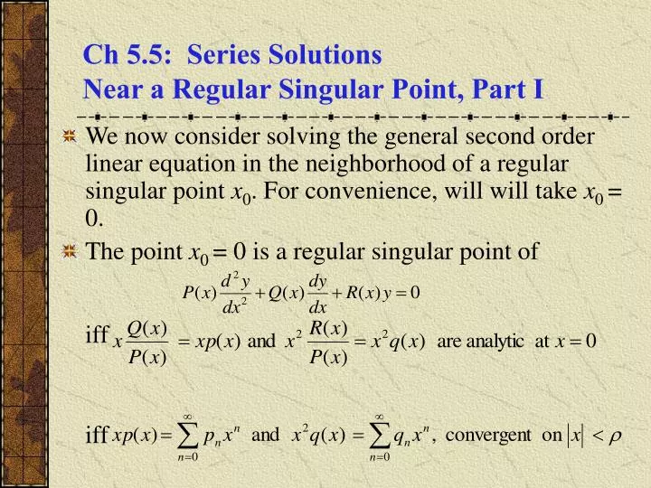
Ch 5.5: Series Solutions Near a Regular Singular Point, Part I. We now consider solving the general second order linear equation in the neighborhood of a regular singular point x 0 . For convenience, will will take x 0 = 0. The point x 0 = 0 is a regular singular point of iff iff.

E N D
Ch 5.5: Series Solutions Near a Regular Singular Point, Part I • We now consider solving the general second order linear equation in the neighborhood of a regular singular point x0. For convenience, will will take x0 = 0. • The point x0 = 0 is a regular singular point of iff iff
Transforming Differential Equation • Our differential equation has the form • Dividing by P(x) and multiplying by x2, we obtain • Substituting in the power series representations of p and q, we obtain
Comparison with Euler Equations • Our differential equation now has the form • Note that if then our differential equation reduces to the Euler Equation • In any case, our equation is similar to an Euler Equation but with power series coefficients. • Thus our solution method: assume solutions have the form
Example 1: Regular Singular Point (1 of 13) • Consider the differential equation • This equation can be rewritten as • Since the coefficients are polynomials, it follows that x = 0 is a regular singular point, since both limits below are finite:
Example 1: Euler Equation (2 of 13) • Now xp(x) = -1/2 and x2q(x) = (1 + x )/2, and thus for it follows that • Thus the corresponding Euler Equation is • As in Section 5.5, we obtain • We will refer to this result later.
Example 1: Differential Equation (3 of 13) • For our differential equation, we assume a solution of the form • By substitution, our differential equation becomes or
Example 1: Combining Series (4 of 13) • Our equation can next be written as • It follows that and
Example 1: Indicial Equation (5 of 13) • From the previous slide, we have • The equation is called the indicial equation, and was obtained earlier when we examined the corresponding Euler Equation. • The roots r1 = 1, r2 = ½, of the indicial equation are called the exponents of the singularity, for regular singular point x = 0. • The exponents of the singularity determine the qualitative behavior of solution in neighborhood of regular singular point.
Example 1: Recursion Relation (6 of 13) • Recall that • We now work with the coefficient on xr+n : • It follows that
Example 1: First Root (7 of 13) • We have • Starting with r1 = 1, this recursion becomes • Thus
Example 1: First Solution (8 of 13) • Thus we have an expression for the n-th term: • Hence for x > 0, one solution to our differential equation is
Example 1: Second Root (10 of 13) • Recall that • When r2 = 1/2, this recursion becomes • Thus
Example 1: Second Solution (11 of 13) • Thus we have an expression for the n-th term: • Hence for x > 0, a second solution to our equation is
Example 1: General Solution (13 of 13) • The two solutions to our differential equation are • Since the leading terms of y1 and y2 are x and x1/2, respectively, it follows that y1 and y2 are linearly independent, and hence form a fundamental set of solutions for differential equation. • Therefore the general solution of the differential equation is where y1 and y2 are as given above.
Shifted Expansions • For the analysis given in this section, we focused on x = 0 as the regular singular point. In the more general case of a singular point at x = x0, our series solution will have the form