Singular Value Decomposition in Text Mining

1. Singular Value Decomposition in Text Mining Ram Akella University of California Berkeley Silicon Valley Center/SC Lecture 4b February 9, 2011

2. Class Outline • Summary of last lecture • Indexing • Vector Space Models • Matrix Decompositions • Latent Semantic Analysis • Mechanics • Example

3. Summary of previous class • Principal Component Analysis • Singular Value Decomposition • Uses • Mechanics • Example swap rates

4. Introduction How can we retrieve information using a search engine?. • We can represent the query and the documents as vectors (vector space model) • However to construct these vectors we should perform a preliminary document preparation. • The documents are retrieved by finding the closest distance between the query and the document vector. • Which is the most suitable distance to retrieve documents?

5. Search engine

6. Document File Preparation • Manual Indexing • Relationships and concepts between topics can be established • It is expensive and time consuming • It may not be reproduced if it is destroyed. • The huge amount of information suggest a more automated system

7. Document File Preparation • Automatic indexing To buid an automatic index, we need to perform two steps: • Document Analysis Decide what information or parts of the document should be indexed • Token analysis Decide with words should be used in order to obtain the best representation of the semantic content of documents.

8. Document Normalization After this preliminary analysis we need to perform another preprocessing of the data • Remove stop words • Function words: a, an, as, for, in, of, the… • Other frequent words • Stemming • Group morphological variants • Plurals “ streets” -> “street” • Adverbs “fully” -> “full” • The current algorithms can make some mistakes • “police“, “policy” -> “polic”

9. File Structures Once we have eliminated the stop words and apply the stemmer to the document we can construct: • Document File • We can extract the terms that should be used in the index and assign a number to each document.

10. File Structures • Dictionary • We will construct a searchable dictionary of terms by arranging them alphabetically and indicating the frequency of each term in the collection

11. File Structures • Inverted List • For each term we find the documents and its related position associated with

12. Vector Space Model • The vector space model can be used to represent terms and documents in a text collection • The document collection of n documents can be represented with a matrix of m X n where the rows represent the terms and the columns the documents • Once we construct the matrix, we can normalize it in order to have unitary vectors

13. Vector Space Models

14. Query Matching • If we want to retrieve a document we should: • Transform the query to a vector • look for the most similar document vector to the query. One of the most common similarity methods is the cosine distance between vectors defined as: Where a is the document and q is the query vector

15. Example: • Using the book titles we want to retrieve books of “Child Proofing” Book titles Query 0 1 0 0 0 1 0 0 Cos 2=Cos 3=0.4082 Cos 5=Cos 6=0.500 With a threshold of 0.5, the 5th and the 6th would be retrieved.

16. Term weighting • In order to improve the retrieval, we can give to some terms more weight than others. Local Term Weights Global Term Weights Where

17. Synonymy and Polysemy auto engine bonnet tyres lorry boot car emissions hood make model trunk make hidden Markov model emissions normalize Synonymy Will have small cosine but are related Polysemy Will have large cosine but not truly related

18. Matrix Decomposition To produce a reduced –rank approximation of the document matrix, first we need to be able to identify the dependence between columns (documents) and rows (terms) • QR Factorization • SVD Decomposition

19. QR Factorization • The document matrix A can be decomposed as below: Where Q is an mXm orthogonal matrix and R is an mX m upper triangular matrix • This factorization can be used to determine the basis vectors for any matrix A • This factorization can be used to describe the semantic content of the corresponding text collection

20. Example A=

21. Example

22. Query Matching • We can rewrite the cosine distance using this decomposition • Where rjrefers to column j of the matrix R

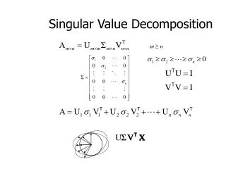
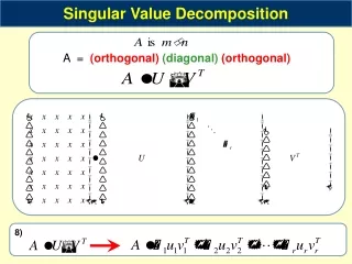
23. mm mn V is nn Singular Value Decomposition (SVD) • This decomposition provides a reduced rank approximations in the column and row space of the document matrix • This decomposition is defined as Where the columns U are orthogonal eigenvectors of AAT. The columns of V are orthogonal eigenvectors of ATA. Eigenvalues 1 … r of AATare the square root of the eigenvalues of ATA.

24. Latent Semantic Decomposition (LSA) • It is the application of SVD in text mining. • We decompose the document-term matrix A into three matrices V A U The V matrix refers to terms and U matrix refers to documents

25. Latent Semantic Analysis • Once we have decomposed the document matrix A we can reduce its rank • We can account for synonymy and polysemy in the retrieval of documents • Select the vectors associated with the higher value of in each matrix and reconstruct the matrix A

26. Latent Semantic Analysis

27. Query Matching • The cosines between the vector q and the n document vectors can be represented as: • where ej is the canonical vector of dimension n This formula can be simplified as where

28. Example Apply the LSA method to the following technical memo titles c1: Human machine interface for ABC computer applications c2: A survey of user opinion of computersystemresponsetime c3: The EPSuserinterface management system c4: System and humansystem engineering testing of EPS c5: Relation of user perceived responsetime to error measurement m1: The generation of random, binary, ordered trees m2: The intersection graph of paths in trees m3: Graphminors IV: Widths of trees and well-quasi-ordering m4: Graphminors: A survey

29. Example First we construct the document matrix

30. Example The Resulting decomposition is the following {U} =

31. Example {S} =

32. Example {V} =

33. Example • We will perform a 2 rank reconstruction: • We select the first two vectors in each matrix and set the rest of the matrix to zero • We reconstruct the document matrix

34. Example The word user seems to have presence in the documents where the word human appears