Download
1 / 51
510 likes | 713 Views
Mining Motifs from Biosequences. Computer Science Department National Chiao Tung University Yuh-Jyh Hu. Outline. Introduction to DNA Sequence Motif Prediction Characteristics of DNA Motif-finding Problem Issues of DNA Motif-finding Algorithms Examples and current research directions

E N D
Mining Motifs from Biosequences Computer Science Department National Chiao Tung University Yuh-Jyh Hu
Outline • Introduction to DNA Sequence Motif Prediction • Characteristics of DNA Motif-finding Problem • Issues of DNA Motif-finding Algorithms • Examples and current research directions • Introduction to RNA Structure Motif Prediction • RNA Secondary Structures • RNA Secondary Structure Prediction Basics • Prediction Methods
What is a sequence motif ? • A subsequence that occurs in multiple sequences with important biological meanings. • Motifs can be totally constants or have variable characters. • Protein motifs often result from structural features, e.g. binding groups in globins. • DNA motifs provide signals for protein binding or nucleic acid bindings. • TRANSFAC database • Holds information of experimentally verified transcription factors.
Characteristics of DNA Motif-finding Problem • Chemical reactions determine gene regulation • Shape of molecules involved • Physicochemical properties of molecules involved • e.g. interaction between regulatory proteins and their target binding sites, expecting local shapes can be primarily determined by the bases involved
Characteristics of DNA Motif-finding Problem • Some evidence supported by the structure of known motifs • Patterns are relatively short — define a local shape • Patterns not defined by an exact sequence of bases • Pattern location may vary in different sequences • Pattern multiplicity is important • Common to most of the sequences in a given family • Motif-finding problem is ill-defined • “motif”, “pattern”, “most”, etc. • Computationally difficult
Issues of DNA Motif-finding Algorithms • Objective function • To approximate the correlation between patterns and biological meanings • Heuristics derived from domain knowledge, e.g., secondary structure of homologous proteins, relation between energetic interactions among bases and base frequencies, etc. • Some proposed objective functions: • Information content • Statistical significance • Generative model, e.g., HMM
Issues of DNA Motif-finding Algorithms • Objective function • Time for using objective functions may vary in different approaches • Some use objective function as heuristics to guide the search for motifs (heuristics applied along with the entire search process) • Some use objective function as a measure to rank the motifs found in the end (heuristics applied only in the end, not during the search) • Many objective functions currently used, but a fact worth notice: • They are all heuristics providing no guarantee. • Statistical significance ≠ biological significance
Issues of DNA Motif-finding Algorithms • Representation • Basic/Simplest: Primary biosequences are described by a double- or single-stranded string of alphabet (nucleotides or amino acids) • Lack flexibility • Motifs can rarely be described by exact strings due to complexity of motif binding mechanism. • IUPAC-IUB code extends expressiveness by including degenerate nucleotides, e.g., R={A,G}. • Capable of presenting unions of nucleotides • Lack base preference information
Issues of DNA Motif-finding Algorithms • Representation • Position weight matrices(PWM) provide base preferences • Each element of the matrix represents a particular base’s occurrence frequency/probability in a specific position of the motif. • Cannot model correlations between bases • Cannot model insertions or deletions 1 2 3 4 5 A 0.4 0.0 0.6 0.1 0.5 G 0.3 0.8 0.4 0.6 0.0 C 0.3 0.1 0.0 0.3 0.0 T 0.0 0.1 0.0 0.0 0.5
Issues of DNA Motif-finding Algorithms • Representation • HMM: a probabilistic model defined over a set of states and transition probabilities. • More expressive than PWM • Can model correlation between bases • Can model insertions and deletions • Require a lot more data to train HMM than other representations
Issues of DNA Motif-finding Algorithms • Representation • Sequence Logos provide graphical summary of conservation of elements in a motif. • Relative heights of letters reflect their frequencies in an alignment. • Entropy-based measurements of conservation
Issues of DNA Motif-finding Algorithms • Representation • Spectrum more efficient less efficient base string IUPAC-IUB PWM HMM less expressive more expressive
Issues of DNA Motif-finding Algorithms • Search Strategy • Closely related to local multiple alignment • To base strings or IUPAC-IUB codes, exhaustive search is applicable. • Limited data set size • Limited motif length • Stochastic approaches • Random sampling • Iterative improvement • No guarantee for optimal solutions
Gibbs Sampling • How Gibbs captures a motif • Probabilistic matrix of a motif with length w • The goal of Gibbs sampling is to maximize the difference between motif base composition and background base distribution.
Gibbs Sampling • Actual locations of motif are unknown beforehand
Gibbs Sampling • First randomly pick motif locations in each sequence
Gibbs Sampling • Take out one sequence at a time with its segment. • Form the motif without a1’ segment.
Gibbs Sampling • Score each segment (in the left-out seq) with the current motif.
Gibbs Sampling • Scoring Gibbs is aimed at optimizing the ratio of motif base composition to background base composition. Maximizing S is equivalent to maximizing F. where Sx: score of motif x W: width of motif ci,j : the count of nucleic base j in position i qi,j : the probability of nucleic base j in position i pi,j:the background probability of nucleic base j in position i pj:the background probability of nucleic base j, which is equal to pi,j
Gibbs Sampling • Score each segment (in the left-out seq) with the current motif.
Gibbs Sampling • Sample a new segment for sequence 1’s motif occurrence according to scores. • Put Sequence 1 back and derive a modified motif.
Gibbs Sampling • Repeat the same process till convergence.
BioProspector • A C program using Gibbs sampling strategy finds DNA sequence motifs with 1-2 blocks. • Challenges • Variable sites per sequence • Motifs may not be highly conserved • Motifs conserved only in a cluster, not in the entire genome • Motifs may have two blocks separated by a gap in variable length. • Sample motif x1 from its marginal distribution • Sample x2 from the conditional distribution on x1
RNA Biological Roles • Like DNA, RNA has 4 bases (AGCU). Less stable than DNA, so is not mainly storage media. • The DNA code of a gene is copied to mRNA. • mRNA is the version of the genetic codes translated at the ribosome. • The ribosome is made up by rRNA. • The individual amino acids are brought to the ribosome, as it reads the mRNA by the molecule called tRNA.
Biological Significance of RNA Folding • RNA takes on 3D structure, and this may affect • Stability within cell • Speed of translation • Frequency of translation • Interactions with other molecules, e.g., regulation of other mRNA.
RNA Secondary Structures • G-C and A-U form hydrogen bonded base pairs and are said to be complementary. • Base pairs are approximately coplanar and are almost always stacked onto other base pairs in an RNA structure. Contiguous base pairs are called stems. • Unlike DNA, RNA is typically produced as a single stranded molecule which then folds intramolecularly to form a number of short base-paired stems. This base-paired structure is called RNA secondary structure.
RNA Secondary Structures • Single stranded subsequences bounded by base pairs are called loops. A loop at the end of a stem is called a hairpin loop. Simple substructures consisting of a simple stem and loop are called stem loops or hairpins. • Single stranded bases within a stem are called a bulge or bulge loop if the single stranded bases are on only one side of the stem. • If single stranded bases interrupt both sides of a stem, they are called an internal (interior) loop. • There are multibranched loops from which three or more stems radiate.
RNA Secondary Structures • Sequences variations in RNA sequences maintain basepairing patterns that give rise to double-stranded regions (secondary structures) in molecules. • Alignments of RNA sequences will show covariation at interacting base-pair positions, see figure below.
RNA Secondary Structures • In addition to secondary structural interactions in RNA, there are also tertiary interactions, illustrated in figure below. These include A. pseudoknots, B. kissing hairpins and C. hairpin-bulge contact. • These complicated structures are usually not predictable by secondary structure prediction tools.
RNA Secondary Structure Prediction Basics • Like protein secondary structure, RNA secondary structure can be viewed as an intermediate step in the formation of a 3D structure. • In predicting RNA secondary structure, several simplifying assumptions are usually made. • The most likely structure is similar to the energetically most stable structure. • The energy associated with any position in the structure is only influenced by local sequence and structure. — most reliable when used for standard Watson-Crick base pairs and single G/U pairs surrounded by Watson-Crick pairs. • The structure is assumed to be formed by folding of the chain back on itself in a manner that does not produce any knots.
Type of RNA Secondary Structure Prediction Methods • Based on objective functions • Free energy minimization • Covariance analysis from sequence comparison • Based on number of RNA sequences for which to predict • Single-sequence prediction • To find the possible folding of a single RNA sequence • Multiple-sequence prediction • To find a global structure alignment for a set of RNA sequences • To find common structure elements within a set of RNA sequences
Prediction Methods • Prediction Based on Self-Complementary Regions • Dot matrix sequence comparison for self-complementary regions • The sequence is listed in the 5’3’ direction across the top of the page, and the complementary strand is listed down the side of the page, also in the 5’3’ direction. The matrix is checked for identities. Self-complementary regions are recognized as diagonal rows of dots, e.g., seq = 5’-CGAAUUUUUCG-3’ seq = 3’-GCUUAAAAAGC-5’ CGAAAUUUUUCG C G A A A A A U U C G
Prediction Methods • Prediction Based on Minimum Free Energy • Based on the observation that the stability of an RNA fold can be decomposed into the contributions of individual energies. • Favorable contributions include: • Hydrogen bonds of basepairs • Stacking interactions of bases • Some ad hoc basepairs created in irregular structures, e.g., loops of 4 bases (i.e. tetraloop) • Unfavorable contributions include: • Symmetric bulges in stems • Asymmetric bulges in stems • Increasing size of loop at the end of stem • Multi-branches from a single loop
Prediction Methods • Prediction Based on Minimum Free Energy • To predict RNA secondary structure, every base is first compared to every other base. The energy of each predicted structure is estimated by the summing the negative base-stacking energies for each pair of bases in double-stranded regions and by adding the estimated positive energies of destabilizing regions such as loops at the end of hairpins, bulges within hairpins, internal bulges, and other unpaired regions. • To evaluate all the different possible structures, a dynamic programming algorithm similar to that used in sequence alignment is applied.
Prediction Methods • Prediction Based on Minimum Free Energy • An example
Prediction Methods • Prediction Based on Sequence Covariation • This method examines columns of a multiple sequence alignment that co-vary to produce base-pairs, i.e., to look for sequence positions at which covariation maintains the base-pairing property. • The justification for this method is that covaritions are actually found to occur during evolution, e.g., using covariation analysis to decipher base-pair interaction in tRNA.
Prediction Methods • COVE (a formal covariance model) • The model is an ordered tree, e.g., (A) SCFG (B) RNA structure (C) parse tree • Successfully identified tRNA genes. • Extremely slow.
Prediction Methods • COVE (a formal covariance model) • To model two RNA hairpins with 3 basepairs and a GGCA or UGCC loop would be: S -> aW1u | uW1a | cW1g | gW1c W1 -> aW2u | uW2a | cW2g | gW2c W2 -> aW3u | uW3a | cW3g | gW3c W3 -> ggca | ugcc • This approach is similar to training a HMM for proteins to recognize a family of protein sequences. In the case of RNA, a tree model is trained by the RNA sequences, and the model is used to predict the most probable secondary structure.
Prediction Methods • GPRM: Genetic Programming for RNA Motifs • What we are dealing with is: • An important but less studied problem: post-transcriptional regulation • Unlike DNA-binding proteins • Sequence conservation v.s. Structure conservation • A set of post-transcriptionally coregulated RNAs • Characterized by basepair interactions • Finding common structural motifs in a family of coregulated RNA sequences
Motif Prediction v.s. Concept Learning • Target concept: common motifs • Training examples: biosequences • Motif prediction as supervised learning: • Positive examples: • a given set of coregulated RNAs • Negative examples: • the same number of sequences randomly generated based on the observedfrequencies of sequence alphabet in positive examples. • Target concept: • The common structural motifs that can be used to distinguish the given coregulated RNAs from the random sequences.
GPRM: Genetic Programming for RNA Motifs • Focus on finding Watson-Crick complementary basepairs • C-G and A-U • RNA secondary structures are typically formed by basepairing interactions. • Three components of GPRM • Population of putative structural motifs • Fitness function of motifs • Genetic operators that simulate the natural evolution process of motifs
Representing Individuals in A Population • Each individual in a population is a putative motif • Structural motif description: • Watson-Crick complementary segments • Non-pairing segments
Fitness Function • Interested in those motifs that can reflect the characteristics conserved in a family of coregulated RNAs • Assign higher values to those motifs commonly shared by the given family of RNAs, and rarely contained in random RNA sequences. • We define the fitness function as:
Genetic Operators • Reproduction • Pass the better half of the population to the next generation • Accelerate the reproduction process • Mutation • If a complementary segment is picked, its segment length and corresponding pairing segment are both randomly changed. • If a non-pairing segment is selected, then only its length is randomly modified. • Crossover • Exchange segment configuration between two putative motifs. • Either a pair of complementary segments or a non-pairing segment is randomly chosen for exchange.