Download
1 / 36
1.01k likes | 2.09k Views
SIMULTANEOUS EQUATION MODELS. ECONOMETRICS DARMANTO STATISTICS UNIVERSITY OF BRAWIJAYA. PREFACE….

E N D
SIMULTANEOUS EQUATION MODELS ECONOMETRICS DARMANTO STATISTICS UNIVERSITY OF BRAWIJAYA
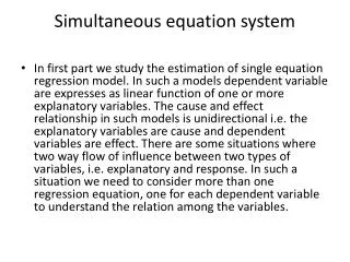
PREFACE… • In contrast to single-equation models, in simultaneous-equation models more than one dependent, or endogenous, variable is involved, necessitating as many equations as the number of endogenous variables. • A unique feature of simultaneous-equation models is that the endogenous variable (i.e., regressand) in one equation may appear as an explanatory variable (i.e., regressor) in another equation of the system. • As a consequence, such an endogenous explanatory variable becomes stochastic and is usually correlated with the disturbance term of the equation in which it appears as an explanatory variable. • In this situation the classical OLS method may not be applied because the estimators thus obtained are not consistent, that is, they do not converge to their true population values no matter how large the sample size.
EXAMPLES : 1.1 • DEMAND-AND-SUPPLY MODEL • As is well known, the price P of a commodity and the quantity Q sold are determined by the intersection of the demand-and-supply curves for that commodity. • Thus, assuming for simplicity that the demand-and-supply curves are linear and adding the stochastic disturbance terms u1 and u2, … (1) … (2)
EXAMPLES : 2.1 • KEYNESIAN MODEL OF INCOME DETERMINATION Consider the simple Keynesian model of income determination: • Consumption function: Ct = β0 + β1Yt + ut ; 0 <β1 < 1 …(3) • Income identity: Yt = Ct + It ( = St ) …(4) • where C = consumption expenditure Y = income I = investment (assumed exogenous) S = savings t = time u = stochastic disturbance term β0 and β1=parameters
EXAMPLES: 3 …(5) …(6)
EXAMPLES: 4 • THE IS MODEL OF MACROECONOMICS The celebrated IS, or goods market equilibrium, model of macroeconomics in its nonstochastic form can be expressed as
EXAMPLES: 5 • ECONOMETRIC MODEL: Klein’s model I (Professor Lawrence Klein of the Wharton School of the University of Pennsylvania). His initial model`is as follows:
THE IDENTIFICATION PROBLEM SIMULTANEOUS EQUATION MODELS
PREFACE… • The problem of identification precedes the problem of estimation. • The identification problem asks whether one can obtain unique numerical estimates of the structural coefficients from the estimated reduced form coefficients. • If this can be done, an equation in a system of simultaneous equations is identified. If this cannot be done, that equation is un- or under-identified. • An identified equation can be just identified or over-identified. In the former case, unique values of structural coefficients can be obtained; in the latter, there may be more than one value for one or more structural parameters.
NOTATION AND DEFINITION: 1 • The general M equations model in M endogenous, or jointly dependent,variables may be written as Eq. (7):
NOTATION AND DEFINITION: 2 • Where Y1, Y2, ... , YM = M endogenous, or jointly dependent, variables X1, X2, ... , XK = K predetermined variables (one of these X variables may take a value of unity to allow for the intercept term in each equation) u1, u2, ... , uM = M stochastic disturbances t = 1, 2, ... , T = total number of observations β’s = coefficients of the endogenous variables γ’s = coefficients of the predetermined variables
NOTATION AND DEFINITION: 3 • The variables entering a simultaneous-equation model are of two types: • Endogenous, that is, those (whose values are) determined within the model; and • Predetermined, that is, those (whose values are) determined outside the model. • The predetermined variables are divided into two categories: • Exogenous, current as well as lagged, and Thus, X1t is a current (present-time) exogenous variable, whereas X1(t−1) is a lagged exogenous variable, with a lag of one time period. • Lagged endogenous. Y(t−1) is a lagged endogenous variable with a lag of one time period, but since the value of Y1(t−1) is known at the current time t, it is regarded as non-stochastic, hence, a predetermined variable.
NOTATION AND DEFINITION: 4 • The equations appearing in (7) are known as the structural, or behavioral, equations because they may portray the structure (of an economic model) of an economy or the behavior of an economic agent (e.g., consumer or producer). • The β’s and γ’s are known as the structural parameters or coefficients. • From the structural equations one can solve for the M endogenous variables and derive the reduced-form equations and the associated reduced form coefficients. • A reduced-form equation is one that expresses an endogenous variable solely in terms of the predetermined variables and the stochastic disturbances.
NOTATION AND DEFINITION: 5 • Consider the simple Keynesian model of income determination: Consumption function: Ct = β0 + β1Yt + ut ; 0 <β1 < 1 …(3) Income identity: Yt = Ct + It ( = St ) …(4) If (3) is substituted into (4), we obtain, after simple algebraic manipulation, …(8) where reduced-form equation …(9) reduced-form coefficient
NOTATION AND DEFINITION: 6 • Substituting the value of Y from (8) into C of (3), we obtain another reduced-form equation: • The reduced-form coefficients, such as ∏1 and ∏3, are also known as impact, or short-run, multipliers, because they measure the immediate impact on the endogenous variable of a unit change in the value of the exogenous variable. …(10) where …(11)
NOTATION AND DEFINITION: 7 • If in the preceding Keynesian model the investment expenditure is increased by, say, $1 and if the MPC is assumed to be 0.8, then from (9) we obtain ∏1 = 5. This result means that increasing the investment by $1 will immediately (i.e., in the current time period) lead to an increase in income of $5, that is, a fivefold increase. • Similarly, under the assumed conditions, (11) shows that ∏3 = 4, meaning that $1 increase in investment expenditure will lead immediately to $4 increase in consumption expenditure.
THE IDENTIFICATION PROBLEM • By the identification problem we mean whether numerical estimates of the parameters of a structural equation can be obtained from the estimated reduced-form coefficients. • If this can be done, we say that the particular equation is identified. • If this cannot be done, then we say that the equation under consideration is unidentified, or under-identified. • An identified equation may be either: • Exactly (or fully or just) identified. if unique numerical values of the structural parameters can be obtained • Over-identified. If more than one numerical value can be obtained for some of the parameters of the structural equations.
UNDER-IDENTIFICATION: 1 • Consider once again the demand-and-supply model (1) and (2), together with the market-clearing, or equilibrium, condition that demand is equal to supply. By the equilibrium condition, we obtain …(12) …(12.a) where …(13) …(14)
UNDER-IDENTIFICATION: 2 • Substituting Pt from (12.1) into (1) or (2), we obtain the following equilibrium quantity: …(15) where …(16) …(17)
UNDER-IDENTIFICATION: 3 • Equations (12.a) and (15) are reduced-form equations. Now our demand-and-supply model contains four structural coefficients α0, α1, β0, and β1, but there is no unique way of estimating them. WHY…? The answer lies in the two reduced-form coefficients given in (13) and (16). These reduced-form coefficients contain all four structural parameters, but there is no way in which the four structural unknowns can be estimated from only two reduced-form coefficients.
JUST OR EXACT IDENTIFICATION: 1 • Consider the following demand-and-supply model • By the market-clearing mechanism we have …(18) …(19) …(20)
JUST OR EXACT IDENTIFICATION: 2 • Solving this equation, we obtain the following equilibrium price: …(21) where …(22)
JUST OR EXACT IDENTIFICATION: 3 • Substituting the equilibrium price into the demand or supply equation, we obtain the corresponding equilibrium quantity: …(23) where …(24)
OVER-IDENTIFICATION • Let modify the demand function (18) as follows, keeping the supply function as before (R represents wealth): …(25) …(26) …(27) …(28) (29)…
RULES OF IDENTIFICATION • Fulfill the order and rank conditions, • Notations: M= number of endogenous variables in the model m = number of endogenous variables in a given equation K= number of predetermined variables in the model including theintercept k= number of predetermined variables in a given equation
THE ORDER CONDITION OF IDENTIFIABILITY: 1 • DEFINITION 1: In a model of M simultaneous equations in order for an equation to be identified, it mustexclude at least M − 1 variables (endogenous as well as pre-determined) appearing in themodel. If it excludes exactly M − 1 variables, the equation is just identified. If it excludes morethan M − 1 variables, it is over-identified. • DEFINITION 2: In a model of M simultaneous equations, in order for an equation to be identified, the numberof pre-determined variables excluded from the equation must not be less than the number ofendogenous variables included in that equation less 1, that is, K − k ≥ m− 1 (...30) If K − k = m − 1, the equation is just identified, but if K − k > m − 1, it is over-identified.
THE RANK CONDITION OF IDENTIFIABILITY: 1 • RANK CONDITION OF IDENTIFICATION In a model containing M equations in M endogenous variables, an equation is identified if andonly if at least one nonzero determinant of order (M − 1)(M − 1) can be constructed from thecoefficients of the variables (both endogenous and predetermined) excluded from that particular equation but included in the other equations of the model.
THE RANK CONDITION OF IDENTIFIABILITY: 2 • Consider thefollowing hypothetical system of simultaneous equations in which the Yvariables are endogenous and the X variables are predetermined • Consider the first equation, which excludes variables Y4, X2, and X3
THE RANK CONDITION OF IDENTIFIABILITY: 3 • The first equation: • Since the determinant is zero, the rank of the matrix, denoted byρ(A), is less than 3. Therefore, Eq. (19.3.2) does not satisfy the rank condition and hence is not identified. • As noted, the rank condition is both a necessary and sufficient conditionfor identification. Therefore, although the order condition shows thatEq. (19.3.2) is identified, the rank condition shows that it is not. Apparently,
THE RANK CONDITION OF IDENTIFIABILITY: 4 • To apply the rank condition one may proceed as follows: • Write down the system in a tabular form • Strike out the coefficients of the row in which the equation underconsideration appears. • Also strike out the columns corresponding to those coefficients in 2which are nonzero. • The entries left in the table will then give only the coefficients of thevariables included in the system but not in the equation under consideration.