Download
1 / 27
270 likes | 403 Views
Variability Indicators in Structural Equation Models. Michael Biderman University of Tennessee at Chattanooga www.utc.edu/Michael-Biderman. Background: Modeling Faking of Personality Tests.

E N D
Variability Indicators in Structural Equation Models Michael Biderman University of Tennessee at Chattanooga www.utc.edu/Michael-Biderman
Background: Modeling Faking of Personality Tests • For the past few years I’ve investigated the utility of a structural equation model of faking of personality questionnaires, specifically the Big Five. • The model is a CFA containing • latent variables representing personality dimensions, and • one or more latent variables representing amount of response distortion, i.e., faking.
The Basic Faking Model E-H A-H C-H E S F C A I S-H O-H HE1 HS1 HC1 HA1 HA2 HE2 HS2 HC2 HS3 HE3 HA3 HC3 HS4 HC4 HE4 HA4 HA5 HE5 HC5 HS5 HO1 HO2 HO3 HO4 HO5 FE1 FE2 FE3 E-D FE4 FE5 A-D FA1 FA2 FA3 C-D FA4 FA5 FC1 S-D FC2 FC3 FC4 O-D FC5 FS1 FS2 FS3 FS4 I FP FA S C A E FS5 FI1 FI2 E-I FI3 C-I FI4 FI5 A-I S-I I-I Applied to two-condition data Applied to three-condition data
Beyond the Basic Model: The basic model represents changes in central tendency associated with faking fairly well. Is that all there is? Last year, during manual data entry of Mike Clark’s thesis data (Yes, UTC is a full-service university) . . . I noticed that some participants seemed to be targeting specific responses, e.g., 6 6 6 6 6 6 Since such targeting results in low variability this suggested the possibility that variability of responding might be an indicator of faking. The following describes an attempt to model variability.
Other studies of variability Traitedness studies (Britt, 1993; Dwight, Wolf & Golden, 2002; Hershberger, Plomin, & Pedersen, 1995). A person is highly traited on a dimension if the variability of responses to items from the dimension is small. Extreme response style (Greenleaf, 1992). Stability of responses to the same scale over time (Eid & Diener, 1999; Kernis, 2005). No studies of variability of responses in faking situations. None of variability and the Big Five.
Three used datasets. • 1: Biderman & Nguyen, 2004. N=203 • 2: Wrensen & Biderman, 2005. N=166 • Two-condition data: Honest and Fake Good • 50 item IPIP Big Five questionnaire given twice • 2-item parcels analyzed • Clark & Biderman, 2006. N=166 • Three-conditions: Honest, Incentive, Instructed faking • Three 30-item IPIP Questionnaires given. • Whole-scale scores analyzed. • Wonderlic Personnel Test (WPT) was given to all participants prior to the first condition.
Measuring Variability To represent variability of responses within dimensions, I computed the standard deviation of responses within each Big Five dimension for each participant for each condition I added the standard deviations as observed variables to the data to which the faking model had previous been applied
SdHE A C S E I F SdHA SdHC SdHS HC1 HS1 HA1 HE1 HC2 HS2 HE2 HA2 SdHI HE3 HC3 HA3 HS3 HS4 HA4 HE4 HC4 HA5 HS5 HE5 HC5 SdFE SdFA SdFC SdFS SdFI HO1 HO2 HO3 HO4 HO5 FE1 FE2 FE3 FE4 FE5 FA1 FA2 FA3 FA4 FA5 FC1 FC2 FC3 FC4 FC5 FS1 FS2 FS3 FS4 FS5 FI1 FI2 FI3 FI4 FI5 Datasets 1 and 2 with Standard Deviations added
E-D A-D C-D S-D O-D E A FA FP I S C E-I C-I A-I S-I I-I Dataset 3 with standard deviations added SdE-H E-H SdA-H A-H SdC-H C-H SdS-H S-H SdO-H O-H SdE-D SdA-D SdC-D SdS-D SdO-D SdE-I SdA-I SdC-I SdS-I SdO-I
Modeling Standard Deviations - 1 Faking leads to elevated central tendency, often resulting in ceiling effects. Ceiling effects lead to lower variability. So the standard deviations were connected to central tendency via regression links. Specifically, standard deviations were regressed onto parcel or scale scores.
A C S E F I HC1 HS1 HE1 HA1 HE2 HS2 HA2 HC2 HE3 HS3 HA3 HC3 HA4 HC4 HE4 HS4 SdHE HC5 HA5 HS5 HE5 SdHA SdHC HO1 HO2 HO3 HO4 HO5 SdHS SdHI FE1 FE2 FE3 FE4 FE5 SdFE FA1 FA2 FA3 FA4 FA5 SdFA FC1 FC2 FC3 FC4 FC5 SdFC FS1 FS2 FS3 FS4 FS5 SdFS FI1 FI2 FI3 FI4 FI5 SdFI Modeling Ceiling Effects in Datasets 1 and 2:Standard deviations were regressed onto parcel scores
SdE-H E-H SdA-H A-H SdC-H C-H SdS-H S-H SdO-H O-H SdE-D E-D A-D SdA-D C-D SdC-D S-D SdS-D O-D SdO-D C FA A I S E FP E-I C-I A-I S-I SdE-I I-I SdA-I SdC-I SdS-I SdO-I Modeling Ceiling Effects in Dataset 3: Standard Deviations regressed onto scale scores
Modeling Standard Deviations - 2 The assumption/hope? was that there are individual differences in variability of responding within dimensions So a latent variable representing such individual differences was added to the model.
. A I S C E V F SdHE . HS1 HC1 HE1 HA1 HE2 HS2 HA2 HC2 HA3 HE3 HC3 HS3 HS4 HE4 HC4 HA4 SdHA HS5 HC5 HA5 HE5 . SdHC . HO1 SdHS . HO2 HO3 HO4 HO5 . SdHI . FE1 SdFE FE2 FE3 FE4 . FE5 FA1 SdFA FA2 FA3 FA4 . FA5 FC1 SdFC FC2 FC3 FC4 FC5 . FS1 SdFS FS2 FS3 FS4 FS5 FI1 SdFI FI2 FI3 FI4 FI5 Modeling variability in Dataset 1 & 2: Adding a “Variability” latent variable
SdE-H E-H SdA-H A-H SdC-H C-H SdS-H S-H SdO-H O-H SdE-D SdA-D SdC-D SdS-D SdO-D E-D A-D C-D S-D SdE-I O-D SdA-I E A C FA FP V S I SdC-I E-I SdS-I C-I SdI-I A-I S-I I-I Modeling variability in Dataset 3: Adding a “Variability” latent variable
Results Did the regression links significantly improve goodness of fit? Are there individual differences in variability of responding that are captured by the V latent variable?
Chi-square difference test of regression links: Χ2(50)=625.685 p<.001 .81 E C A S I V F .26 .16 SHE -.06 .69 HE1 HC1 HS1 HA1 .28 HC2 HA2 HS2 HE2 .37 Chi-square difference test of V latent variable: Χ2(16)=218.041 p<.001 HA3 HC3 HE3 HS3 HS4 HA4 HC4 HE4 .38 SHA HS5 HA5 HC5 HE5 -.14 .72 .10 .31 .34 .31 SHC -.14 .79 .50 .27 .52 HI1 SHS -.07 .60 HI2 HI3 .47 .08 HI4 HI5 .37 SHI -.11 .36 .30 .38 FE1 SFE -.07 FE2 .17 FE3 FE4 .27 .30 .27 FE5 FA1 .08 SFA FA2 -.16 FA3 .42 .35 FA4 .50 .31 FA5 .44 FC1 .34 SFC -.16 FC2 .62 FC3 FC4 .60 FC5 .22 .34 .50 FS1 SFS FS2 -.09 FS3 FS4 FS5 .45 FI1 SFI FI2 -.09 FI3 FI4 FI5 ΔΧ2(31)=597.537 p<.001 Results of application of Variability model to Dataset 1 Model Χ2(1539)=2501.249; p<.001; CFI=.871; RMSEA=.055 Both the regression links and the V latent variable improved model fit.
Chi-square difference test of regression links: ΔΧ2(50)=747.249 p<.001 .75 E V F A I S C .14 .01 SHE -.08 .67 HC1 HS1 HA1 HE1 .02 HA2 HE2 HC2 HS2 .23 HC3 HE3 HA3 HS3 Chi-square difference test of V latent variable: ΔΧ2(16)=274.468 p<.001 HE4 HC4 HA4 HS4 .31 SHA HS5 HA5 HC5 HE5 -.16 .70 -.07 .23 .28 .52 SHC -.14 .75 .20 .26 .39 HO1 SHS -.06 .63 HO2 HO3 .35 .02 HO4 HO5 .26 SHO -.14 .38 .20 .42 FE1 SFE -.13 FE2 .08 FE3 FE4 .19 -.01 .56 FE5 FA1 .05 SFA FA2 -.20 FA3 .36 .00 FA4 .50 .26 FA5 .51 FC1 .40 SFC -.19 FC2 .67 FC3 FC4 .63 FC5 .25 .25 .56 FS1 SFS FS2 -.09 FS3 FS4 FS5 .46 FO1 SFO FO2 -.18 FO3 FO4 FO5 ΔΧ2(31)=608.423 p<.001 Results of application of Variability model to Dataset 2 Model Χ2(1539)=2666.874; p<.001; CFI=.816; RMSEA=.066 Again, both the regression links and the V latent variable improve model fit.
SdE-H E-H Chi-square difference test of regression links: ΔΧ2(15)=268.367 p<.001 SdA-H A-H -.09 SdC-H C-H .73 SdS-H S-H SdO-H O-H .47 .62 SdE-D ΔΧ2(12)=37.910 p<.05 SdA-D 43 -.24 .52 .38 SdC-D .16 SdS-D SdO-D Chi-square difference test of V latent variable: ΔΧ2(22)=405.333 p<.001 .26 .29 .26 .41 ΔΧ2(17)=260.217 p<.001 (FP correlations with Big 5 LVs set at 0 for this test.) .57 SdE-I .35 SdA-I -.43 .67 SdC-I .11 SdS-I .31 SdI-I .19 .26 E-D A-D C-D S-D O-D FP FA V E A C S I E-I C-I A-I S-I I-I Results of application of Variability model to Dataset 3 Model Χ2(352)=532.552; p<.001; CFI=.883; RMSEA=.056
Tentative Conclusions regarding Variability Model 1) Ceiling effects seem to be successfully modeled by the regressions of standard deviations onto parcels or scale scores. 2) Individual differences in variability of responding to items within dimensions seem to be captured by the V latent variable. Some persons consistently exhibited little variability in responding to items within questionnaire scales. Others exhibit greater variability in responding.
What about V and faking? 1) Loadings on V might be larger in faking conditions – magnifying individual differences in variability because some people are targeting while others are not. Mean Standardized Loadings of Standard Deviation indicators on V Dataset 1 HonestIncentive to fakeInstructed to fake Mean loading .406 .366 Dataset 2 HonestIncentive to fakeInstructed to fake Mean loading .411 .496 Dataset 3 HonestIncentive to fakeInstructed to fake Mean loading .468 .521 .413 Tentative Conclusion: Loadings on V are approximately equal in honest and faking conditions.
What about V and faking? 2) V might be related to the faking latent variables. Dataset 1: Correlation of V with F: .04 NS Dataset 2: Correlation of V with F: .02 NS Dataset 3: Correlation of V with FP: .16 NS Correlation of V with FA: .10 NS It appears from these preliminary analyses that variability of responding is not related to faking However, other scenarios and models should be explored
What is V? 1) Perhaps V is related to personality characteristics It appears that V has discriminant validity with respect to the Big Five.
What is V? 2) Perhaps V is related to cognitive ability These results suggest that persons with higher CA exhibit less variability of responding.
FA V I Dataset 1: Multiple R = .57 Dataset 2: Multiple R = .35 Dataset 3: Multiple R = .50 e WPT Uses of V How about using it to extract cognitive ability from the Big Five? The structural model suggests that there is information on cognitive ability embedded in “noncognitive” personality tests.
Conclusions • 1) V appears to be an individual difference variable that cuts across personality dimensions. • V appears to be unrelated to faking • 3) V appears to be independent of the Big Five dimensions. • 4) V appears to be related to cognitive ability – persons higher in cognitive ability have lower variability of responding
Implications Don’t throw away old datasets. You never know what constructs may be hidden in them.