Use of Geostationary Satellite Observations for Dynamical Support of Model Cloud Fields

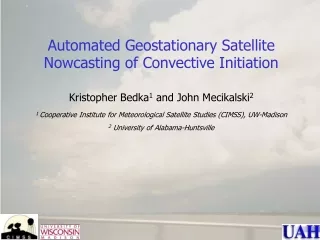
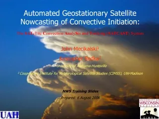
1. Use of Geostationary Satellite Observations for Dynamical Support of Model Cloud Fields • Arastoo Pour Biazar1, Richard T. McNider1, Kevin Doty1, Yun-Hee Park1, Maudood Khan2, Bright Dornblaser3 • University of Alabama in Huntsville • The Universities Space Research Association • Texas Commission on Environmental Quality (TCEQ) • Presented at • 9th Annual CMAS Conference, October 11-13, 2010 • Friday Center, UNC-Chapel Hill

2. Motivation Use of Satellite Data to Improve the Prediction of Clouds in Air Quality Decision Models • The uncertainties in physical atmosphere such as temperature, moisture, winds, and cloud prediction greatly impact air quality model predictions. e.g., clouds have an important role in regulating the photochemical reaction rates, heterogeneous chemistry, and the evolution and partitioning of particulate matter. • Numerical meteorological models have traditionally had significant problems in creating clouds in the right place and time compared to observed clouds. This is especially the case during air pollution episodes when synoptic-scale forcing is weak. • The initiation and assimilation of clouds in weather forecast models has been the subject of many investigations. Yet, cloud prediction remains a pervasive problem and evidence suggests that there are still major errors in cloud placement. This is especially true at the spatial scale at which air quality models operate. • The problem in cloud prediction is particularly frustrating in air quality SIP modeling since they are retrospective simulations in which the observed cloud field is known from satellite observations but models have significant differences in cloud placement. • The overall purpose of the current effort is to improve model location and timing of clouds in the Weather Research and Forecast (WRF) meteorological model which is widely used in the air quality planning community.

3. Background • At UAH considerable attention has been given to the use of geostationary satellite observations to improve the representation of physical atmosphere in the air quality simulations. • One such effort has been replacing model cloud transmissivity with satellite observed transmissivity in air quality models. However, while this technique provided improvements in model performance, it produced a physical inconsistency in the model system. Insolation and photolysis fields were derived from satellite data, but deep convection or cloud venting of the boundary layer or the impact of cloud water on long wave radiation or chemistry could be in the wrong location according to model placement of clouds. • The new activity attempts to create an environment in the model conducive to creating clouds where there are observed clouds and remove clouds where the observations indicate clear sky. • Previous attempts at using satellite data to insert cloud water have met with limited success. Previous studies have also indicated that adjustment of the model dynamics and thermodynamics is necessary to fully support the insertion of cloud liquid water in models. • Our approach is to develop relationships between satellite-derived cloud properties and targeted variables internal to the model such as grid scale vertical velocity and to provide the dynamical and thermodynamical support needed to sustain or clear model clouds. • This technique was first implemented in MM5 and we are in the process of transitioning it to WRF. WE are also pursuing a simple alternative threshold approach.

4. ASSIMILATION OF GOES-DERIVED CLOUD PRODUCTS IN MM5 Satellite Model/Satellite comparison Underprediction W<0 W>0 0.65um VIS surface, cloud features Overprediction • Use satellite cloud top temperatures and cloud albedoes to determine a maximum vertical velocity (Wmax) in the cloud column (Multiple Linear Regression). • Adjust divergence to comply with Wmax in a way similar to O’Brien (1970). • Nudge MM5 winds toward new horizontal wind field to sustain the vertical motion. • Remove erroneous model clouds by imposing subsidence and suppressing convective initiation.

5. Total Cloud Depth Number of Cloud Layers Depth Wmax Layer Wmax Height of Wmax Est. 1-h stable precip. Est. 1-h convective precip. Height of Max. Diabatic Heating Magnitude of Maximum Diabatic Heating Layer with Upward Motion Satellite Products Multiple Linear Regression Variables • Cloud Albedo • Cloud Top Pressure / Brightness Temperature • Short Wave Radiation • Surface Albedo • Skin Temperature

6. Satellite Observation Control Run Assimilation Surface incident shortwave radiation in W m-2 for July 2, 1999. Assimilation and satellite observation plots are @ 14:45 UTC, and the control run is @ 15:00 UTC. Control: Control run with no assimilation. Assimilation: Run with assimilation of satellite cloud information. Satellite Observation: Derived from GOES–8 satellite.

7. SATELLITE DATA IS UTILIZED TO CORRECT MODEL CLOUD FIELDS IN A DYNAMICALLY CONSISTENT MANNER Downward shortwave radiation in W m-2 at 2200 UTC 6 July 1999. (A) Derived from GOES–8 satellite. (B) Control run with no assimilation. (C) Run with assimilation of satellite cloud information. Satellite OBSERVEDInsolation MODEL CNTRL A MODEL ASSIMILATION B C

8. BIAS = (Total model predicted cloud) / (Total observed cloud) Series 1: control simulation;Series 2: satellite assimilation

9. MM5 PAUSE: WRITE SPECIAL HISTORY CALCULATE ZHMAX CALCULATE MAXIMUM HEATING INTERPOLATE/ AVERAGE BACK TO MM5 GRID WRITE OUT NUDGING FILES CALL PROGRAM WADJ ESTIMATE PRECIP RATES DETERMINE STABLE/CONV. CATEGORY ADD NEW DIVERGENT COMPONENTS MM5 CONTINUE READ MM5, SATELLITE, SFC DATA CALCULATE ZWMAX DO STABLE ADJUSTMENT CALCULATE NEW DIVERGENT COMPONENTS Flowchart showing the flow of the processes needed for cloud adjustment at each hour Way to complicated and computationally expensive for operational use INTERPOLATE TO SIGMA-H GRID CHECK FOR PRIOR WMAX DO CONVECTIVE ADJUSTMENT ADJUST DIVERGENCE FOR WMAX CLUSTER ANALYSES CALCULATE WMAX REMOVE ERRONEOUS CLOUDS SUBTRACT ORIGINAL DIVERGENT COMPONENTS CALCULATE TOTAL CLOUD DEPTH CALCULATE WMAX CLOUD DEPTH DETERMINE NUDGING TIME SCALES CALCULATE ORIGINAL DIVERGENT COMPONENTS REMOVE SHALLOW CLOUDS CALCULATE NUMBER OF CLOUD LAYERS CALCULATE UPWARD DEPTH CALCULATE ORIGINAL DIVERGENCE

10. The Way Forward • Two different tracks are followed: • Streamline the current technique and implement it in WRF. • Clearing erroneous clouds are more difficult in WRF. WRF’s response to suppressing the convective parameterization is different from MM5 (WRF compensate by creating grid resolved clouds). • Revisit the problem and develop a simpler approach. • Focusing on daytime clouds, revisit the relationship between internal model cloud variables and relate them to what satellite can observe. • Case study: summer of 2006; WRF configuration: 36-km grid spacing, CONUS with 42 vertical layers; SW radiation: Dudhia; LW radiation: RRTM; Monin_Obukhov similarity with NOAH LSM; PBL scheme: YSU; Microphysics: Lin; Cumulus parameterization: Kain-Fritsch; IC/BC/nudging: EDAS.

11. Use of Daytime Cloud Albedo/Cloud Top Temperature for Model Evaluation Model Cloud Albedo Satellite Cloud Albedo 0.65um VIS surface, cloud features 10.7um IR sfc/cloud top temperature

12. Areas of Underprediction/Overprediction can be identified for Correction Model cloud top temperature Model cloud albedo Underprediction Areas of disagreement between model and satellite observation Overprediction

13. Evaluating Model Cloud Prediction During August 2006 Agreement Index (AI) =(Clear/Cloudy agreements) / (Total Number of Grids) Weak Synoptic-scale forcing Increased cloudiness over the domain Overprediction Underprediction

14. Model Cloud, W, and Relative Humidity positive W cloud albedo Functional relationships between cloud water and/or cloud albedo with model vertical motion was not clear. Thus, threshold relationships with vertical motion and relative humidity were examined. A contingency probability approach, where the coincidence of clouds/clear occurring with positive/negative vertical motion were examined. RH < 95% RH > 95%

15. Alternative Simple Approach for Creating Dynamical Support for Clouds Threshold Table for target W (August 2006 Simulation) • Obtain threshold vertical velocities and moisture needed to support cloud formation from WRF. • From GOES observations identify the areas of cloud under-/over-prediction and use the threshold information to obtain the needed vertical velocity in the model to achieve agreement with observations. • Having the threshold vertical velocity as the target, use one dimensional variational technique to calculate new divergence fields and target horizontal winds. • Use the new horizontal winds and threshold moisture fields as nudging fields in WRF to sustain the target vertical velocity.

16. Preliminary Results From 1D-Variational Scheme Original wind field @ 25th layer A Snapshot of the Modified Wind Field For August 19. Color filled contours represent vertical velocity. Horizontal wind fields were modified to sustain the target vertical velocity. New wind field

17. Preliminary Results Control WRF simulation: August 19, 2006, 20 GMT Satellite assimilation: August 19, 2006, 20 GMT

18. CONCLUSION & FUTURE WORK • Statistical relationships between clouds and WRF model variables were examined. While functional relationships were not clear, an examination of coincident relations showed that threshold relations between vertical motion and relative humidity were very robust. • 98% of the model cloudy grids were associated with positive vertical motions and over 65% of the grids with clear condition were associated with negative vertical motions. This largely confirms the working hypothesis that in a GOES black and white image, white areas are associated with lifting and negative areas with subsidence. • The statistics suggested that imposing positive/negative vertical velocity can create/clear clouds where there are inconsistencies with GOES observation. • Preliminary results from the use of threshold vertical velocities are encouraging. • The results presented here are preliminary and the technique needs further refinements. Coincidently, relative humidity will be adjusted below clouds to be consistent with model statistics.

19. Acknowledgment The findings presented here were accomplished under partial support from NASA Science Mission Directorate Applied Sciences Program and the Texas Commission on Environmental Quality (TCEQ). Note the results in this study do not necessarily reflect policy or science positions by the funding agencies.