Download
1 / 16
160 likes | 270 Views
A Holy Grail for stellar wind analysis zeta Puppis seen by XMM. Y. Nazé (FNRS-ULg), G. Rauw (ULg), L. Oskinova (U. Potsdam), E. Gosset (FNRS-ULg), A. Hervé (ULg), C.A. Flores (U. Guanajuato). Zeta Puppis. One of the closest (335pc), earliest (O4I), and brightest massive stars

E N D
A Holy Grail for stellar wind analysis zeta Puppis seen by XMM Y. Nazé (FNRS-ULg), G. Rauw (ULg), L. Oskinova (U. Potsdam), E. Gosset (FNRS-ULg), A. Hervé (ULg), C.A. Flores (U. Guanajuato)
Zeta Puppis • One of the closest (335pc), earliest (O4I), and brightest massive stars • Many intriguing properties : runaway star, chemical enrichment, fast rotation (post RLOF+SN ? Ejection from cluster ?) • The first one observed by Chandra & XMM (Kahn et al. 2001, Cassinelli et al. 2011)
A decade of XMM observations • 18 observations
Data reduction • The best dataset available for a massive star (~1/2 Ms for EPIC, 3/4 Ms for RGS) • 18 observations taken in different modes (timing, full frame, large window, small window), with different filters (medium, thick), sometimes off-axis • Bright slight pile-up (~limit of large window mode) • Extraction with pattern=0, keeping the same circular regions for source and bkgd (NB: annular source = KO!) • New RGS pipeline (SAS 10) solved the flux/shift issues
Variability of zeta Puppis • In optical : • long-term changes (Conti & Niemela 1976) • 5d variations (e.g. Moffat & Michaud 1981) • a few h pulsations (e.g. Reid & Howarth 1996) • In X-rays : • Einstein - nothing • ROSAT revealed a small modulation (2% amplitude) of 17h period in 0.9-2 keV band (Berghöfer et al. 1996) • Chandra, XMM (1 dataset) – nothing (Kahn et al. 2001, Oskinova et al. 2001)
Variability: the XMM view • Several energy bands • Several time bins (200s to 5ks EPIC, 500s to 10ks RGS) • Chi-2 tests (constant, line, parabola); Fourier; Autocorrelation • Results : • Background is variable • Instruments do not agree
Variability: short & mid-term • The longer you observe or the longer the time bin, the more variable it is no obvious short term variations but mid-term ones exist (with timescales > Texp : rotation ?)
Variability: short and mid-term For the best data (small window, thick filter) • Fourier • 0.3-0.4/d + ~1/d ? • Rotation (5d) ???? • Autocorrelation • >0 if T<20ks, <0 @ 55ks • wind flow time ~5ks Not very significant anyway Best case : pn data
Variability: lines • RGS data • TVS : nothing • Count rates and ratios : nothing • Comparison with average spectrum by eye : non-significant variations may exist but similar to optical…
Variability: long-term • EPIC, RGS : decrease ! • NB : Fourier, autocorrelation and relative dispersions calculated after detrending
Variability: long-term • EPIC spectra : fitted by tbabs (ISM, fixed) * sum of 4 thermal comp. (vphabs*vapec – Nh and kT fixed) • Pile-up affects all data taken with medium filter • Formally unacceptable fitting but missing physics and disagreement between instruments • Flux appears quite constant (a few % decrease?) count rate variations come from detector sensitivity changes
A simple model • Features (Oskinova et al. 2004) • smooth wind or random absorbers • random emitters • solid angle conserved, outward motion (beta law) • LCs less variable: • at high E • for smooth wind • For more emitting/absorbing clumps
How to compare with data? • Relative dispersions calculated for each observation • for full LCs • for resampled LCs • Poisson noise ! • Relative dispersions in both cases ~ Poisson statistics ! If additional variability exists, it is hidden in noise… hence its amplitude is small, and emitting/absorbing clumps are many (>105) !
Global spectral fitting : preliminary results • a (Kahn et al. 2001, Cassinelli et al. 2011)
Line fitting : preliminary results • Line profile fitting using Owocki & Cohen models : variation of tau with wavelength (cf. Cohen et al. 2010, in green – NB with resonance scattering in red) BUT /!\ uniqueness of solution…
Conclusions • A decade of XMM observations = best dataset ! • Variability • Only noise on short-term • Trends on mid-term (DACs ? But no link with rotation, cf. Fourier) • Long-term decrease due to detector degradation • Comparison with models : a lot of wind parcels needed ! • Lines • Multi-temperature needed • Typical optical depth varies with wavelength • For the future… • Follow the star over its rotation period • Observe it with more sensitive detectors to decrease Poisson noise • Develop more detailed models