Download
1 / 59
590 likes | 643 Views
Clustering Chapter 7. TexPoint fonts used in EMF. Read the TexPoint manual before you delete this box.: A A A A A A A. Rating. Area maturity Practical importance Theoretical importance. First steps Text book.

E N D
ClusteringChapter 7 TexPoint fonts used in EMF. Read the TexPoint manual before you delete this box.: AAAAAAA
Rating • Area maturity • Practical importance • Theoretical importance First steps Text book No apps Mission critical Not really Must have
Overview • Motivation • Dominating Set • Connected Dominating Set • General Algorithms: • The “Greedy” Algorithm • The “Tree Growing” Algorithm • The “Marking” Algorithm • The “k-Local” Algorithm • Algorithms for Special Models: • Unit Ball Graphs: The “Largest ID” Algorithm • Bounded Independence Graphs: The “MIS” Algorithm • Unstructured Radio Network Model
Motivation • In theory clustering is the solution to almost any problem in ad hoc and sensor networks. It improves almost any algorithm, e.g. in data gathering it selects cluster heads which do the work while other nodes can save energy by sleeping. Here, however, we motivate clustering with routing: • There are thousands of routing algorithms… • Q: How good are these routing algorithms?!? Any hard results? • A: Almost none! Method-of-choice is simulation… • Flooding is key component of (many) proposed algorithms, including most prominent ones (AODV, DSR) • At least flooding should be efficient
Backbone • Idea: Some nodes become backbone nodes (gateways). Each node can access and be accessed by at least one backbone node. • Routing: • If source is not agateway, transmitmessage to gateway • Gateway acts asproxy source androutes message onbackbone to gatewayof destination. • Transmission gatewayto destination.
(Connected) Dominating Set • A Dominating Set DS is a subset of nodes such that each node is either in DS or has a neighbor in DS. • A Connected Dominating Set CDS is a connected DS, that is, there is a path between any two nodes in CDS that does not use nodes that are not in CDS. • A CDS is a good choicefor a backbone. • It might be favorable tohave few nodes in the CDS. This is known as theMinimum CDS problem
Formal Problem Definition: M(C)DS • Input: We are given an (arbitrary) undirected graph. • Output: Find a Minimum (Connected) Dominating Set,that is, a (C)DS with a minimum number of nodes. • Problems • M(C)DS is NP-hard • Find a (C)DS that is “close” to minimum (approximation) • The solution must be local (global solutions are impractical for mobile ad-hoc network) – topology of graph “far away” should not influence decision who belongs to (C)DS
Greedy Algorithm for Dominating Sets • Idea: Greedilychoose “good” nodes into the dominating set. • Black nodes are in the DS • Grey nodes are neighbors of nodes in the DS • White nodes are not yet dominated, initially all nodes are white. • Algorithm: Greedily choose a node that colors most white nodes. • One can show that this gives a log approximation, if is the maximum node degree of the graph. (The proof is similar to the “Tree Growing” proof on the following slides.) • One can also show that there is no polynomial algorithm with better performance unless P¼NP.
CDS: The “too simple tree growing” algorithm • Idea: start with the root, and then greedily choose a neighbor of the tree that dominates as many as possible new nodes • Black nodes are in the CDS • Grey nodes are neighbors of nodes in the CDS • White nodes are not yet dominated, initially all nodes are white. • Start: Choose a node with maximum degree, and make it the root of the CDS, that is, color it black (and its white neighbors grey). • Step: Choose a grey node with a maximum number of white neighbors and color it black (and its white neighbors grey).
Example of the “too simple tree growing” algorithm Graph with 2n+2 nodes; tree growing: |CDS|=n+2; Minimum |CDS|=4 tree growing: start … Minimum CDS u u u v v v
Tree Growing Algorithm • Idea: Don’t scan one but two nodes! • Alternative step: Choose a grey node and its white neighbor node with a maximum sum of white neighbors and color both black (and their white neighbors grey).
Analysis of the tree growing algorithm • Theorem: The tree growing algorithm finds a connected set of size |CDS| · 2(1+H()) ¢ |DSOPT|. • DSOPT is a (not connected) minimum dominating set • is the maximum node degree in the graph • H is the harmonic function with H(n) ¼ log(n)+0.7 • In other words, the connected dominating set of the tree growing algorithm is at most a O(log()) factor worse than an optimum minimum dominating set (which is NP-hard to compute). • With a lower bound argument (reduction to set cover) one can show that a better approximation factor is impossible, unless P¼NP.
Proof Sketch • The proof is done with amortized analysis. • Let Su be the set of nodes dominated by u 2 DSOPT, or u itself. If a node is dominated by more than one node, we put it in one of the sets. • We charge the nodes in the graph for each node we color black. In particular we charge all the newly colored grey nodes. Since we color a node grey at most once, it is charged at most once. • We show that the total charge on the vertices in an Su is at most 2(1+H()), for any u.
Charge on Su • Initially |Su| = u0. • Whenever we color some nodes of Su, we call this a step. • The number of white nodes in Su after step i is ui. • After step k there are no more white nodes in Su. • In the first step u0 – u1 nodes are colored (grey or black). Each vertex gets a charge of at most 2/(u0 – u1). • After the first step, node u becomes eligible to be colored (as part of a pair with one of the grey nodes in Su). If u is not chosen in step i (with a potential to paint ui nodes grey), then we have found a better (pair of) node. That is, the charge to any of the new grey nodes in step i in Su is at most 2/ui. u
Discussion of the tree growing algorithm • We have an extremely simple algorithm that is asymptotically optimal unless P¼NP. And even the constants are small. • Are we happy? • Not really. How do we implement this algorithm in a real mobile network? How do we figure out where the best grey/white pair of nodes is? How slow is this algorithm in a distributed setting? • We need a fully distributed algorithm. Nodes should only consider local information.
The Marking Algorithm • Idea: The connected dominating set CDS consists of the nodes that have two neighbors that are not neighboring. 1. Each node u compiles the set of neighbors N(u) • Each node u transmits N(u), and receives N(v) from all its neighbors • If node u has two neighbors v,w and w is not in N(v) (and since the graph is undirected v is not in N(w)), then u marks itself being in the set CDS. + Completely local; only exchange N(u) with all neighbors + Each node sends only 1 message, and receives at most + Messages have size O() • Is the marking algorithm really producing a connected dominating set? How good is the set?
Correctness of Marking Algorithm • We assume that the input graph G is connected but not complete. • Note: If G was complete then constructing a CDS would not make sense. Note that in a complete graph, no node would be marked. • We show: The set of marked nodes CDS is a) a dominating set b) connected c) a shortest path in G between two nodes of the CDS is in CDS
Proof of a) dominating set • Proof: Assume for the sake of contradiction that node u is a node that is not in the dominating set, and also not dominated. Since no neighbor of u is in the dominating set, the nodes N+(u) := u [ N(u) form: • a complete graph • if there are two nodes in N(u) that are not connected, u must be in the dominating set by definition • no node v 2 N(u) has a neighbor outside N(u) • or, also by definition, the node v is in the dominating set • Since the graph G is connected it only consists of the complete graph N+(u). We precluded this in the assumptions, therefore we have a contradiction
Proof of b) connected, c) shortest path in CDS • Proof: Let p be any shortest path between the two nodes u and v, with u,v 2 CDS. • Assume for the sake of contradiction that there is a node w on this shortest path that is not in the connected dominating set. • Then the two neighbors of w must be connected, which gives us a shorter path. This is a contradiction. w u v
Improved Marking Algorithm • If neighbors with larger ID are connected and cover all other neighbors, then don’t join CDS, else join CDS 9 2 6 8 5 4 1 7 3
Correctness of Improved Marking Algorithm • Theorem: Algorithm computes a CDS S • Proof (by induction of node IDs): • assume that initially all nodes are in S • look at nodes u in increasing ID order and remove from S if higher-ID neighbors of u are connected • S remains a DS at all times: (assume that u is removed from S) • S remains connected:replace connection v-u-v’ by v-n1,…,nk-v’ (ni: higher-ID neighbors of u) u lower-ID neigbors higher-ID neighbors higher-ID neighbors cover lower-ID neighbors
Quality of the (Improved) Marking Algorithm • Given an Euclidean chain of n homogeneous nodes • The transmission range of each node is such that it is connected to the k left and right neighbors, the id’s of the nodes are ascending. • An optimal algorithm (and also the tree growing algorithm) puts every k’th node into the CDS. Thus |CDSOPT| ¼ n/k; with k = n/c for some positive constant c we have |CDSOPT| = O(1). • The marking algorithm (also the improved version) does mark all the nodes (except the k leftmost ones). Thus |CDSMarking| = n – k; with k = n/c we have |CDSMarking| = (n). • The worst-case quality of the marking algorithm is worst-case!
Algorithm Overview Input: Local Graph Fractional Dominating Set Dominating Set Connected Dominating Set 0.2 0.2 0 0.5 0.3 0 0.8 0.3 0.5 0.1 0.2 Phase B: Probabilistic algorithm Phase C: Connect DS by “tree” of “bridges” Phase A: Distributed linear program rel. high degree gives high value
Phase A is a Distributed Linear Program • Nodes 1, …, n: Each node u has variable xuwith xu¸ 0 • Sum of x-values in each neighborhood at least 1 (local) • Minimize sum of all x-values (global) 0.5+0.3+0.3+0.2+0.2+0 = 1.5 ¸ 1 • Linear Programs can be solved optimally in polynomial time • But not in a distributed fashion! That’s what we need here… Linear Program 0.2 0.2 0 0.5 0.3 0 0.8 0.3 0.5 0.1 0.2 Adjacency matrix with 1’s in diagonal
Result after Phase A • Distributed Approximation for Linear Program • Instead of the optimal values xi* at nodes, nodes have xi(), with • The value of depends on the number of rounds k (the locality) • The analysis is rather intricate…
Phase B Algorithm Each node applies the following algorithm: • Calculate (= maximum degree of neighbors in distance 2) • Become a dominator (i.e. go to the dominating set) with probability • Send status (dominator or not) to all neighbors • If no neighbor is a dominator, become a dominator yourself Highest degree in distance 2 From phase A
Result after Phase B • Randomized rounding technique • Expected number of nodes joining the dominating set in step 2 is bounded by log(+1) ¢ |DSOPT|. • Expected number of nodes joining the dominating set in step 4 is bounded by |DSOPT|. • Phase C essentially the same result for CDS Theorem:
v 1 u Better and faster algorithm • Assume that graph is a unit disk graph (UDG) • Assume that nodes know their positions (GPS)
Then… transmission radius
Grid Algorithm • Beacon your position • If, in your virtual grid cell, you are the node closest to the center of the cell, then join the DS, else do not join. • That’s it. • 1 transmission per node, O(1) approximation. • If you have mobility, then simply “loop” through algorithm, as fast as your application/mobility wants you to.
k-local algorithm Algorithm computes DS k2+O(1) transmissions/node O(O(1)/klog ) approximation General graph No position information Grid algorithm Algorithm computes DS 1transmission/node O(1) approximation Unit disk graph (UDG) Position information (GPS) Comparison The model determines the distributed complexity of clustering
General Graph Captures obstacles Captures directional radios Often too pessimistic UDG & GPS UDG is not realistic GPS not always available Indoors 2D 3D? Often too optimistic Let’s talk about models… too pessimistic too optimistic Let‘s look at models in between these extremes!
The “Largest-ID” Algorithm • All nodes have unique IDs, chosen at random. • Algorithm for each node: • Send ID to all neighbors • Tell node with largest ID in neighborhood that it has to join the DS • Algorithm computes a DS in 2 rounds (extremely local!) 7 6 1 4 2 9 10 5 8 3
“Largest ID” Algorithm, Analysis I • To simplify analysis: assume graph is UDG(same analysis works for UBG based on doubling metric) • We look at a disk S of diameter 1: S Nodes inside S have distance at most 1. ! they form a clique Diameter: 1 How many nodes in S are selected for the DS?
“Largest ID” Algorithm, Analysis II • Nodes which select nodes in S are in disk of radius 3/2 whichcan be covered by S and 20 other disks Si of diameter 1(UBG: number of small disks depends on doubling dimension) S 1 1 1
“Largest ID” Algorithm: Analysis III • How many nodes in S are chosen by nodes in a disk Si? • x = # of nodes in S, y = # of nodes in Si: • A node u2S is only chosen by a node in Si if (all nodes in Si see each other). • The probability for this is: • Therefore, the expected number of nodes in S chosen by nodes in Si is at most: Because at most y nodes in Si can choose nodes in S and because of linearity of expectation.
“Largest ID” Algorithm, Analysis IV • From x·n and y·n, it follows that: • Hence, in expectation the DS contains at most nodesper disk with diameter 1. • An optimal algorithm needs to choose at least 1 node in the disk with radius 1 around any node. • This disk can be covered by a constant (9) number of disks of diameter 1. • The algorithm chooses at most times more disks than an optimal one
“Largest ID” Algorithm, Remarks • For typical settings, the “Largest ID” algorithm produces very good dominating sets (also for non-UDGs) • There are UDGs where the “Largest ID” algorithm computes an -approximation (analysis is tight). complete sub-graph • Optimal DS: size 2 • “Largest ID” alg: • bottom nodes choose top nodes with probability¼1/2 • 1 node every 2nd group • nodes nodes complete sub-graph
Iterative “Largest ID” Algorithm • Assume that nodes know the distances to their neighbors:all nodes are active;for i := k to 1 do8 act. nodes: select act. node with largest ID in dist. · 1/2i; selected nodes remain activeod;DS = set of active nodes • Set of active nodes is always a DS (computing CDS also possible) • Number of rounds: k • Approximation ratio n(1/2k) • For k=O(loglog n), approximation ratio = O(1)
Iterative “Largest ID” Algorithm, Remarks • Possible to do everything in O(1) rounds(messages get larger, local computations more complicated) • If we slightly change the algorithm such that largest radius is 1/4: • Sufficient to know IDs of all neighbors, distances to neighbors, and distances between adjacent neighbors • Every node can then locally simulate relevant part of algorithm to find out whether or not to join DS UBG w/ distances: O(1) approximation in O(1) rounds
Maximal Independent Set I • Maximal Independent Set (MIS):(non-extendable set of pair-wise non-adjacent nodes) • An MIS is also a dominating set: • assume that there is a node v which is not dominated • vMIS, (u,v)E ! uMIS • add v to MIS
Maximal Independent Set II • Lemma:On bounded independence graphs: |MIS| · O(1)¢|DSOPT| • Proof: • Assign every MIS node to an adjacent node of DSOPT • u2DSOPT has at most f(1) neighbors v2MIS • At most f(1) MIS nodes assigned to every node of DSOPT |MIS| · f(1)¢|DSOPT| • Time to compute MIS on bounded-independence graphs: • Deterministically • Randomized
MIS (DS) CDS MIS gives a dominating set. But it is not connected. Connect any two MIS nodes which can be connected by one additional node. Connect unconnected MIS nodes which can be conn. by two additional nodes. This gives a CDS! #2-hop connectors·f(2)¢|MIS| #3-hop connectors·2f(3)¢|MIS| |CDS| = O(|MIS|)
Models General Graph UDG No GPS UDG GPS too optimistic too pessimistic Unit Ball Graph Quasi UDG Bounded Independence Message Passing Models Physical Signal Propagation Radio Network Model too simplistic too “tough” Unstructured Radio Network Model
Unstructured Radio Network Model • Multi-Hop • No collision detection • Not even at the sender! • No knowledge about (the number of) neighbors • Asynchronous Wake-Up • Nodes are not woken up by messages ! • Unit Disk Graph (UDG)to model wireless multi-hop network • Two nodes can communicate iff Euclidean distance is at most 1 • Upper bound n for number of nodes in network is known • This is necessary due to (n / log n) lower bound [Jurdzinski, Stachowiak, ISAAC 2002]