Download
1 / 49
490 likes | 653 Views
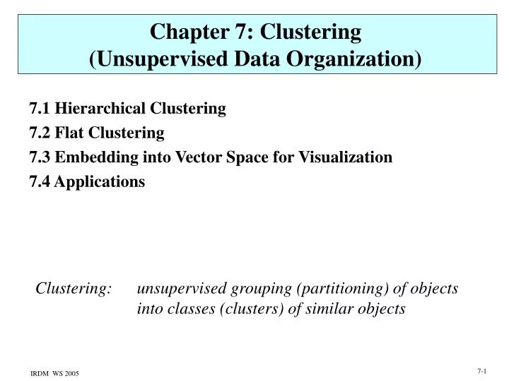
Chapter 7: Clustering (Unsupervised Data Organization). 7.1 Hierarchical Clustering 7.2 Flat Clustering 7.3 Embedding into Vector Space for Visualization 7.4 Applications. Clustering: unsupervised grouping (partitioning) of objects into classes (clusters) of similar objects.

E N D
Chapter 7: Clustering(Unsupervised Data Organization) 7.1 Hierarchical Clustering 7.2 Flat Clustering 7.3 Embedding into Vector Space for Visualization 7.4 Applications Clustering: unsupervised grouping (partitioning) of objects into classes (clusters) of similar objects
Clustering Search Resultsfor Visualization and Navigation http://www.grokker.com/
Example for Hierarchical Clustering dendrogram
Clustering: Classification based onUnsupervised Learning given: n m-dimensional data records dj D dom(A1) ... dom(Am) with attributes Ai (e.g. term frequency vectors N0 ... N0) or n data points with pair-wise distances (similarities) in a metric space wanted: k clusters c1, ..., ck and an assignment D {c1, ..., ck} such that the average intra-cluster similarity is high and the average inter-cluster similarity is low, where the centroid of ck is:
Desired Clustering Properties A clustering function fd maps a dataset D onto a partitioning 2D of D, with pairwise disjoint members of and xD f(x) = D, based on a (metric or non-metric) distance function d: DDR0+ which is symmetric and satisfies d(x,y)=0 x=y Axiom 1: Scale-Invariance For any distance function d and any >0: fd(x) = fd (x) for all xD Axiom 2: Richness (Expressiveness) For every possible partitioning of D there is a distance function d such that fd produces Axiom 3: Consistency d is a -transformation of d if for all x,y in same S : d‘(x,y) d(x,y) and for all x, y in different S, S‘ : d‘(x,y) d(x,y). If fd produces then fd‘ produces , too. Impossibility Theorem (J. Kleinberg: NIPS 2002): For each dataset D with |D|2 there is no clustering function f that satisfies Axioms 1,2, and 3 for every possible choice of d
Hierarchical vs. Flat Clustering • Hierarchical Clustering: • detailed and insightful • hierarchy built • in natural manner • from fairly simple algorithms • relatively expensive • no prevalent algorithm • Flat Clustering: • data overview & coarse analysis • level of detail depends • on the choice of the • number of clusters • relatively efficient • K-Means and EM are simple • standard algorithms
7.1 Hierarchical Clustering:Agglomerative Bottom-up Clustering (HAC) • Principle: • start with each di forming its own singleton cluster ci • in each iteration combine the most similar clusters ci, cj • into a new, single cluster for i:=1 to n do ci := {di} od; C := {c1, ..., cn}; /* set of clusters */ while |C| > 1 do determine ci, cj C with maximal inter-cluster similarity; C := C – {ci, cj} {ci cj}; od;
Principle: • start with a single cluster that contains all data records • in each iteration identify the least „coherent“ cluster • and divide it into two new clusters Divisive Top-down Clustering c1 := {d1, ..., dn}; C := {c1}; /* set of clusters */ while there is a cluster cj C with |cj|>1 do determine ci with the lowest intra-cluster similarity; partition ci into ci1 and ci2 (i.e. ci = ci1 ci2 and ci1 ci2 = ) such that the inter-cluster similarity between ci1 and ci2 is minimized; od; For partitioning a cluster one can use another clustering method (e.g. a bottom-up method)
Alternative Similarity Metrics for Clusters given: similarity on data records - sim: DDR oder [0,1] define: similarity between clusters – sim: 2D2DR or [0,1] • Alternatives: • Centroid method: sim (c,c‘) = sim(d, d‘) with centroid d of c • and centroid d‘ of c‘ • Single-Link method: sim(c,c‘) = sim(d, d‘) with d c, d‘c‘, • such that d and d‘ have the highest similarity • Complete-Link method:sim(c,c‘) = sim(d, d‘) with d c, d‘c‘, • such that d and d‘ have the lowest similarity • Group-Average method: For hierarchical clustering the following axiom must hold: max {sim(c,c‘), sim(c,c‘‘)} sim(c, c‘ c‘‘) for all c, c‘, c‘‘ 2D
Example for Bottom-up Clustering with Single-Link Metric (Nearest Neighbor) run-time: O(n2) with space O(n2) a b c d 5 4 3 2 e f g h 1 1 2 3 4 5 6 7 8 emphasizes „local“ cluster coherence (chaining effect) • tendency towards long clusters
Example for Bottom-up Clustering with Complete-Link Metric (Farthest Neighbor) run-time: O(n2 log n) with space O(n2) a b c d 5 4 3 2 e f g h 1 1 2 3 4 5 6 7 8 emphasizes „global“ cluster coherence • tendency towards round clusters with small diameter
Relationship to Graph Algorithms • Single-Link clustering: • corresponds to construction of maximum (minimum) spanning tree • for undirected, weighted graph G = (V,E) with V=D, E=DD • and edge weight sim(d,d‘) (dist(d,d‘)) for (d,d‘)E • from the maximum spanning tree the cluster hierarchy can be derived • by recursively removing the shortest (longest) edge Single-Link clustering is related to the problem of finding maximal connected components (Zusammenhangskomponenten) on a graph that contains only edges (d,d‘) for which sim(d,d‘) is above some threshold Complete-Link clustering is related to the problem of finding maximal cliques in a graph.
Bottom-up Clustering with Group-Average Metric (1) Merge step combines those clusters ci and cj for which the intra-cluster similarity c: = ci cj becomes maximal naive implementation has run-time O(n3): n-1 merge steps each with O(n2) computations
Bottom-up Clustering with Group-Average Metric (2) efficient implementation – with total run-time O(n2) – for cosine similarity with length-normalized vectors, i.e. using scalar product for sim precompute similarity of all document pairs and compute for each cluster after every merge step Then: Thus each merge step can be carried out in constant time.
Cluster Quality Measures (1) With regard to ground truth: known class labels L1, …, Lg for data points d1, …, dn: L(di) = Lj{L1, …, Lg} With cluster assignment (d1), …, (dn) c1, …, ck cluster cj has purity Complete clustering has purity • Alternatives: • Entropywithin cluster • MIbetween cluster and classes
Cluster Quality Measures (2) Without any ground truth: ratio of intra-cluster to inter-cluster similarities or other cluster validity measures of this kind (e.g. considering variance of intra- and inter-cluster distances)
7.2 Flat Clustering: Simple Single-Pass Method given: data records d1, ..., dn wanted: (up to) k clusters C:={c1, ..., ck} C := {{d1}}; /* random choice for the first cluster */ for i:=2 to n do determine cluster cj C with the largest value of sim(di, cj) (e.g. sim(di, ) with centroid ); if sim(di, cj) threshold then assign di to cluster cj else if |C| < k then C := C {{di}}; /* create new cluster */ else assign di to cluster cj fi fi od
K-Means Method for Flat Clustering (1) • Idea: • determine k prototype vectors, one for each cluster • assign each data record to the most similar prototype vector • and compute new prototype vector • (e.g. by averaging over the vectors assigned to a prototype) • iterate until clusters are sufficiently stable randomly choose k prototype vectors while not yet sufficiently stable do for i:=1 to n do assign di to cluster cj for which is minimal od; for j:=1 to k do od; od;
Example for K-Means Clustering K=2 data records prototype vectors a b a b 5 5 c c 4 4 3 3 d d 2 2 e f e f 1 1 1 2 3 4 5 6 8 1 2 3 4 5 6 8 7 7 after 1st iteration after 2nd iteration
K-Means Method for Flat Clustering (2) • run-time is O(n) (assuming constant number of iterations) • a suitable number of clusters, K, can be determined experimentally • or based on the MDL principle • the initial prototype vectors could be chosen by using another • – very efficient – clustering method • (e.g. bottom-up clustering on random sample of the data records). • for sim any arbitrary metric can be used
Choice of K (Model Selection) • application-dependent (e.g. for visualization) • driven by empirical evaluation of cluster quality • (e.g. cross-validation with held-out labeled data) • driven by quality measure without ground truth • driven by MDL principle
LSI and pLSI Reconsidered • LSI and pLSI can also be seen as • unsupervised clustering methods (spectral clustering): • simple variant for k clusters • map each data point into k-dimensional space • assign each point to its highest-value dimension • (strongest spectral component) Conversely, we could compute k clusters for the data points (using any clustering algorithm) and project data points onto k centroid vectors („axes“ of k-dim. space) to represent data in LSI-style manner
EM Method for Model-based Soft Clustering(Expectation Maximization) • Approach: • generalize K-Means method such that each data record • belongs to a cluster (actually all k clusters) with a certain probability • based on a parameterized multivariate prob. distribution f • random variable Zij = 1 if di belongs to cj, 0 otherwise • estimate parameters of the prob. distribution f(,x) such that • the likelihood that the observed data is indeed a sample from • this distribution is maximized Maximum-Likelihood Estimation (MLE): maximize L(d1,...,dn, ) = P[d1, ..., dn is a sample from f(,x)] or maximize log L; if analytically intractable use EM iteration procedure Postulate probability distribution e.g. mixture of k multivariate Normal distributions
EM Clustering Method with Mixture of kMultivariate Normal Distributions Assumption: data records are a sample from a mixture of k multivariate Normal distributions with the density: with expectation values and invertible, positive definite, symmetric mm covariance matrices maximize log-likelihood function:
EM Iteration Procedure (1) introduce latent variables Zij: point xi generated by cluster j initialization of EM method, for example, by: setting 1=...= k=1/k, using K-Means cluster centroids for and unity matrices (1s on diagonal) for 1, ..., k • iterate until parameter estimations barely change anymore: • Expectation step (E step): • compute E[Zij] based on the previous round‘s estimation • for , i.e. 1, ..., k, and 1, ..., k • 2)Minimization step (M step): • improve parameter estimation for based on • the previous round‘s values for E[Zij] convergence is guaranteed, but may result in local maximum of log-likelihood function
Expectation step (E step): EM Iteration Procedure (2) Maximization step (M step):
given: n=20 terms from articles of the New York Times: ballot, polls, Gov, seats, profit, finance, payments, NFL, Reds, Sox, inning, quarterback, score, scored, researchers, science, Scott, Mary, Barbara, Edward with m=20-dimensional feature vectors with dij = # articles that contain both term i and term j Example for EM Clustering Method Result of EM clustering for the estimation of hij for k=5: 1 2 3 4 5 ballot 0.63 0.12 0.04 0.09 0.11 polls 0.58 0.11 0.06 0.10 0.14 Gov 0.58 0.12 0.03 0.10 0.17 seats 0.55 0.14 0.08 0.08 0.15 profit 0.11 0.59 0.02 0.14 0.15 finance 0.15 0.55 0.01 0.13 0.16 payments 0.12 0.66 0.01 0.09 0.11 NFL 0.13 0.05 0.58 0.09 0.16 Reds 0.05 0.01 0.86 0.02 0.06 Sox 0.05 0.01 0.86 0.02 0.06 1 2 3 4 5 inning 0.03 0.01 0.93 0.01 0.02 quarterback 0.06 0.02 0.82 0.03 0.07 score 0.12 0.04 0.65 0.06 0.13 scored 0.08 0.03 0.79 0.03 0.07 researchers 0.08 0.12 0.02 0.68 0.10 science 0.12 0.12 0.03 0.54 0.19 Scott 0.12 0.12 0.11 0.11 0.54 Mary 0.10 0.10 0.05 0.15 0.59 Barbara 0.15 0.11 0.04 0.12 0.57 Edward 0.16 0.18 0.02 0.12 0.51
Clustering with Density Estimator Influence function influence of data record y on a point x in its local environment e.g. with Density function density at point x: sum of all influences y on x clusters correspond to local maxima of the density function
Example for Clustering with Density Estimator Source: D. Keim and A. Hinneburg, Clustering Techniques for Large Data Sets, Tutorial, KDD Conf. 1999
Incremental DBSCAN Methodfor Density-based Clustering [Ester et al.: KDD 1996] DBSCAN = Density-Based Clustering for Applications with Noise simplified version of the algorithm: for each data point d do { insert d into spatial index (e.g., R-tree); locate all points with distance to d < max_dist; if these points form a single cluster then add d to this cluster else { if there are at least min_points data points that do not yet belong to a cluster such that for all point pairs the distance < max_dist then construct a new cluster with these points }; }; average run-time is O(n * log n); data points that are added later can be easily assigned to a cluster; points that do not belong to any cluster are considered „noise“
similar to K-Means but embeds data and clusters in a low-dimensional space (e.g. 2D) and aims to preserve cluster-cluster neighborhood – for visualization (recall: clustering does not assume a vector space, only a metric space) 7.3 Self-Organizing Maps (SOMs, Kohonen Maps) clusters c1, c2, ... and data x1, x2, ... are points with distance function sim (xi, xj), sim (ci, xj), sim (ci, cj) initialize map with k cluster nodes arbitrarily placed (often on a triangular or rectangular grid) for each x determine node C(x) closest to x and small node set N(x) close to x repeat for randomly chosen x update all nodes c‘N(x): under influence of data point x (with learning rate (t)) („data activates neuron C(x) and other neurons c‘ in its neighborhood“) until sufficient convergence (with gradually reduced (t)) assign data point x to the closest cluster („winner neuron“)
SOM Example (1) from http://www.cis.hut.fi/ research/som-research/worldmap.html see also http://maps.map.net/ for another - interactive - example
SOM Example (2): WWW Map (2001) Source: www.antarcti.ca, 2001
SOM Example (3): Hyperbolic Visualization Source: J. Ontrup, H. Ritter: Hyperbolic Self-Organizing Maps for Semantic Navigation, NIPS 2001
SOM Example (4): „Islands of Music“ Source: E. Pampalk: Islands of Music: Analysis, Organization, and Visualization of Music Archives, Master Thesis, Vienna University of Technology http://www.ofai.at/~elias.pampalk/music/
Multi-dimensional Scaling (MDS) Goal: map data (from metric space) into low-dimensional vector space such that the distances of data xi are approximately preserved by the Euclidean distances of the images = f(xi) in the vector space minimize stress = • solve iteratively with hill climbing: start with random (or heuristic) placement of data in vector space find point pair with highest tension move points locally so as to reduce the stress (on a fictitious spring that connects the points) O(n2) run-time in each iteration, impractical for very large data sets
Idea: pretend that the data are points in an unknown n-dim. vector space and project them into a k-dimensional space by determining their coordinates in k rounds, one dimension at a time FastMap • Algorithm: • determine two pivot objects a and b (e.g. objects far apart) • conceptually project all data points x onto the line between a and b • solve for x1: (cosine law) consider (n-1)-dim. hyperplane perpendicular to the projection line with new distances: (Pythagoras) recursively call FastMap for (n-1)-dimensional data
7.4 Applications:Cluster-based Information Retrieval • for user query q: • compute ranking of cluster centroids with regard to q • evaluate query q on the cluster or clusters • with the most similar centroid(s) • (possibly in conjunction with relevance feedback by user) cluster browsing: user can navigate through cluster hierarchy each cluster ck is represented by its medoid: the document d‘ ck for which the sum is maximal (or has highest similarity to cluster centroid)
Automatic Labeling of Clusters • Variant 1: • classification of cluster centroid • with a separate, supervised, classifier • Variant 2: • using term or terms with the highest • (tf*idf-) weight in the cluster centroid • Variant 2‘: • computing an approximate centroid based • on m‘ (m‘ << m) terms with the highest weights in the cluster‘s docs • and using the highest-weight term or terms of • Variant 3: • identifying most characteristic terms or phrases for each cluster, • using MI or other entropy measures
Clustering Query Logs • Motivation: • statistically identify FAQs (for intranets and portals), • taking into account variations in query formulation • capture correlation between queries and subsequent clicks Model/Notation: a user session is a pair (q, D+) with a query q and D+ denoting the result docs on which the user clicked; len(q) is the number of keywords in q
Similarity Measures between User Sessions • tf*idf based similarity between query keywords only • edit distance based similarity: sim(p,q) = 1 – ed(p,q) / max(len(p),len(q)) Examples: Where does silk come from? Where does dew come from? How far away is the moon? How far away is the nearest star? • similarity based on common clicks: Example: atomic bomb, Manhattan project, Nagasaki, Hiroshima, nuclear weapon • similarity based on common clicks and document hierarchy: p=law of thermodynamics D+p = {/Science/Physics/Conservation Laws, ...} q=Newton law D+q = {/Science/Physics/Gravitation, ...} with • linear combinations of different similarity measures
Query Expansion based on Relevance Feedback Given: a query q, a result set (or ranked list) D, a user‘s assessment u: D {+, } yielding positive docs D+D and negative docs DD Goal: derive query q‘ that better captures the user‘s intention or a better suited similarity function, e.g., by - changing weights in the query vector or - changing weights for different aspects of similarity (color vs. shape in multimedia IR, different colors, relevance vs. authority vs. recency) Classical approach: Rocchio method (for term vectors) with , , [0,1] and typically > >
Pseudo-Relevance Feedback based on J. Xu, W.B. Croft: Query expansion using local and global document analysis, SIGIR Conference, 1996 Lazy users may perceive feedback as too bothersome Evaluate query and simply view top n results as positive docs: Add these results to the query and re-evaluate or Select „best“ terms from these results and expand the query
on MS Encarta corpus, with 4 Mio. query log entries and 40 000 doc. subset Experimental Evaluation Considers short queries and long phrase queries, e.g.: Michael Jordan Michael Jordan in NBA matches genome project Why is the genome project so crucial for humans? Manhattan project What is the result of Manhattan project on Word War II? Windows What are the features of Windows that Microsoft brings us? (Phrases are decomposed into N-grams that are in dictionary) Query expansion with related terms/phrases: Avg. precision [%] at different recall values: Short queries: Long queries: Recall q alone PseudoRF Query Log (n=100,m=30) (m=40) 10% 40.67 45.00 62.33 20% 27.00 32.67 44.33 30% 20.89 26.44 36.78 100% 8.03 13.13 17.07 Recall q alone PseudoRF Query Log (n=100,m=30) (m=40) 10% 46.67 41.67 57.67 20% 31.17 34.00 42.17 30% 25.67 27.11 34.89 100% 11.37 13.53 16.83
S. Chakrabarti, Chapter 4: Similarity and Clustering • C.D. Manning / H. Schütze, Chapter 14: Clustering • R.O. Duda / P.E. Hart / D.G. Stork, Ch. 10: Unsupervised Learning and Clustering • M.H. Dunham, Data Mining, Prentice Hall, 2003, Chapter 5: Clustering • D. Hand, H. Mannila, P. Smyth: Principles of Data Mining, MIT Press, • 2001, Chapter 9: Descriptive Modeling • M. Ester, J. Sander: Knowledge Discovery in Databases, • Springer, 2000, Kapitel 3: Clustering • C. Faloutsos: Searching Multimedia Databases by Content, 1996, Ch. 11:FastMap • M. Ester et al.: A density-based algorithm for discovering clusters in • large spatial databases with noise, KDD Conference, 1996 • J. Kleinberg: An impossibility theorem for clustering, NIPS Conference, 2002 • G. Karypis, E.-H. Han: Concept Indexing: A Fast Dimensionality Reduction Algorithm with Applications to Document Retrieval & Categorization, CIKM 2000 • M. Vazirgiannis, M. Halkidi, D. Gunopulos: Uncertainty Handling and Quality • Assessment in Data Mining, Springer, 2003 • Ji-Rong Wen, Jian-Yun Nie, Hong-Jiang Zhang: Query Clustering Using • User Logs, ACM TOIS Vol.20 No.1, 2002 • Hang Cui, Ji-Rong Wen, Jian-Yun Nie, Wei-Ying Ma: Query Expansion by • Mining User Logs, IEEE-CS TKDE 15(4), 2003 Additional Literature for Chapter 7